3.8: Fermi’s Golden Rule

A number of important relationships in quantum mechanics that describe rate processes come from first-order perturbation theory. These expressions begin with two model problems that we want to work through:

1. time evolution after applying a step perturbation, and
2. time evolution after applying a harmonic perturbation.

As before, we will ask: if we prepare the system in the state \(| \ell \rangle\), what is the probability of observing the system in state \(| k \rangle\) following the perturbation?

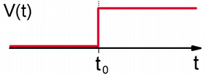
Constant Perturbation (or a Step Perturbation)

The system is prepared such that \(| \psi ( - \infty ) \rangle = | \ell \rangle\). A constant perturbation of amplitude \(V\) is applied at \(t_o\):

\[V (t) = V \Theta \left( t - t _ {0} \right) = \left\{\begin{array} {l l} {0} & {t < t _ {0}} \\ {V} & {t \geq t _ {0}} \end{array} \right. \label{2.148}\]

Here \(\Theta \left( t - t _ {0} \right)\) is the Heaviside step response function, which is 0 for \(t < t_o\) and 1 for \(t ≥ t_0\). Now, turning to first order perturbation theory, the amplitude in \(k \neq \ell\), we have:

\[b _ {k} = - \frac {i} {\hbar} \int _ {t _ {0}}^{t} d \tau \,e^{i \omega _ {k l} \left( \tau - t _ {0} \right)} V _ {k \ell} ( \tau ) \label{2.149}\]

Here \(V_{k\ell}\) is independent of time.

Setting \(t_o = 0\)

\[ \begin{align} b _ {k} &= - \frac {i} {\hbar} V _ {k \ell} \int _ {0}^{t} d \tau \,e^{i \omega _ {k \ell} \tau} \\[4pt] &= - \frac {V _ {k \ell}} {E _ {k} - E _ {\ell}} \left[ \exp \left( i \omega _ {k l} t \right) - 1 \right] \\[4pt] &= - \frac {2 i V _ {k \ell} e^{i \omega _ {k t} t / 2}} {E _ {k} - E _ {\ell}} \sin \left( \omega _ {k t} t / 2 \right) \label{2.150} \end{align}\]

For Equation \ref{2.150}, the following identity was used

\[e^{i \theta} - 1 = 2 i e^{i \theta / 2} \sin ( \theta / 2 ).\]

Now the probability of being in the \(k\) state is

\[ \begin{align} P _ {k} &= \left| b _ {k} \right|^{2} \\[4pt] &= \frac {4 \left| V _ {k \ell} \right|^{2}} {\left| E _ {k} - E _ {\ell} \right|^{2}} \sin^{2} \left( \frac {\omega _ {k \ell} t} {2} \right) \label{2.151} \end{align}\]

If we write this using the energy splitting variable we used earlier:

\[\Delta = \left( E _ {k} - E _ {t} \right) / 2\]

then

\[P _ {k} = \frac {V^{2}} {\Delta^{2}} \sin^{2} ( \Delta t / \hbar ) \label{2.152}\]

Fortunately, we have the exact result for the two-level problem to compare this approximation to

\[P _ {k} = \frac {V^{2}} {V^{2} + \Delta^{2}} \sin^{2} \left( \sqrt {\Delta^{2} + V^{2}} t / \hbar \right) \label{2.153}\]

From comparing Equation \ref{2.152} and \ref{2.153}, it is clear that the perturbation theory result works well for \(V \ll \Delta\), as expected for this approximation approach.

Let’s examine the time-dependence to \(P_k\), and compare the perturbation theory (solid lines) to the exact result (dashed lines) for different values of \(\Delta\).

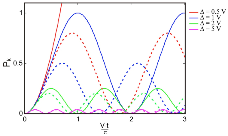
The worst correspondence is for \(\Delta=0.5\) (red curves) for which the behavior appears quadratic and the probability quickly exceeds unity. It is certainly unrealistic, but we do not expect that the expression will hold for the “strong coupling” case: \(\Delta \ll V\). One begins to have quantitative accuracy in for the regime \(P _ {k} (t) - P _ {k} ( 0 ) < 0.1\) or \(\Delta < 4V\).

Now let’s look at the dependence on \(\Delta\). We can write the first-order result Equation \ref{2.152} as

\[P _ {k} = \frac {V^{2} t^{2}} {\hbar^{2}} \text{sinc}^{2} ( \Delta t / 2 \hbar ) \label{2.154}\]

where

\[\text{sinc} (x) = \dfrac{\sin (x)}{x}.\]

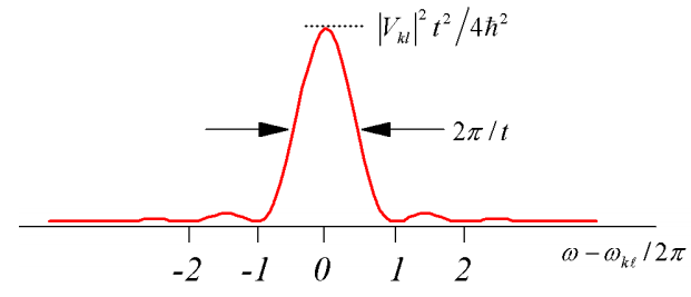
If we plot the probability of transfer from \(| \ell \rangle\) to \(| k \rangle\) as a function of the energy level splitting (\(E_k-K_{\ell}\)), we have:

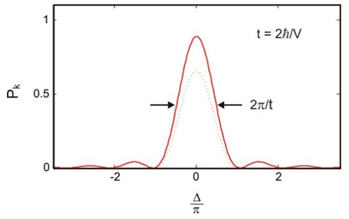
The probability of transfer is sharply peaked where energy of the initial state matches that of the final state, and the width of the energy mismatch narrows with time. Since

\[\lim _ {x \rightarrow 0} \operatorname {sinc} (x) = 1,\]

we see that the short time behavior is a quadratic growth in \(P_k\)

\[\lim _ {\Delta \rightarrow 0} P _ {k} = \dfrac{V^{2} t^{2}}{\hbar^{2}} \label{2.155}\]

The integrated area grows linearly with time.

Uncertainty

Since the energy spread of states to which transfer is efficient scales approximately as \(E _ {k} - E _ {\ell} < 2 \pi \hbar / t\), this observation is sometimes referred to as an uncertainty relation with

\[\Delta E \cdot \Delta t \geq 2 \pi \hbar\]

However, remember that this is really just an observation of the principles of Fourier transforms. A frequency can only be determined as accurately as the length of the time over which you observe oscillations. Since time is not an operator, it is not a true uncertainly relation like

\[\Delta p \cdot \Delta x \geq 2 \pi \hbar.\]

In the long time limit, the \(\text{sinc}^2 (x)\) function narrows to a delta function:

\[\lim _ {t \rightarrow \infty} \frac {\sin^{2} ( a x / 2 )} {a x^{2}} = \frac {\pi} {2} \delta (x) \label{2.156}\]

So the long time probability of being in the \(k\) state is

\[\lim _ {t \rightarrow \infty} P _ {k} (t) = \frac {2 \pi} {\hbar} \left| V _ {k \ell} \right|^{2} \delta \left( E _ {k} - E _ {\ell} \right) t \label{2.157}\]

The delta function enforces energy conservation, saying that the energies of the initial and target state must be the same in the long time limit. What is interesting in Equation \ref{2.157} is that we see a probability growing linearly in time. This suggests a transfer rate that is independent of time, as expected for simple first-order kinetics:

\[w _ {k} (t) = \frac {\partial P _ {k} (t)} {\partial t} = \frac {2 \pi \left| V _ {k \ell} \right|^{2}} {\hbar} \delta \left( E _ {k} - E _ {\ell} \right) \label{2.158}\]

This is one statement of Fermi’s Golden Rule—the state-to-state form—which describes relaxation rates from first-order perturbation theory. We will show that this rate properly describes long time exponential relaxation rates that you would expect from the solution to

\[\dfrac{d P}{d t} = - w P.\]

Harmonic Perturbation

The second model calculation is the interaction of a system with an oscillating perturbation turned on at time \(t_0 = 0\). The results will be used to describe how a light field induces transitions in a system through dipole interactions.

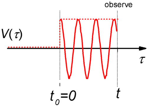
Again, we are looking to calculate the transition probability between states \(\ell\) and \(k\):

\[V (t) = V \cos \omega t \Theta (t) \label{2.159}\]

\[ \begin{align} V _ {k \ell} (t) &= V _ {k \ell} \cos \omega t \label{2.160} \\[4pt] &= \frac {V _ {k \ell}} {2} \left[ e^{- i \omega t} + e^{i \omega t} \right] \end{align}\]

Setting \(t _ {0} \rightarrow 0\), first-order perturbation theory leads to

\[ \begin{align} b _ {k} &= \frac {- i} {\hbar} \int _ {t _ {0}}^{t} d \tau\, V _ {k \ell} ( \tau ) e^{i \omega _ {k l} \tau} \\[4pt] &= \frac {- i V _ {k \ell}} {2 \hbar} \int _ {0}^{t} d \tau \left[ e^{i \left( \omega _ {k l} - \omega \right) \tau} + e^{i \left( \omega _ {k l} + \omega \right) \tau} \right] \\[4pt] &= \frac {- i V _ {k \ell}} {2 \hbar} \left[ \frac {e^{i \left( \omega _ {k l} - \omega \right) t} - 1} {\omega _ {k \ell} - \omega} + \frac {e^{i \left( \omega _ {k t} + \omega \right) t} - 1} {\omega _ {k \ell} + \omega} \right] \end{align} \]

Using

\[e^{\theta} - 1 = 2 i e^{i \theta / 2} \sin ( \theta / 2 )\]

as before:

\[b _ {k} = \frac {V _ {k \ell}} {\hbar} \left[ \underbrace{\frac {e^{i \left( \omega _ {k \ell} - \omega \right) t / 2} \sin \left[ \left( \omega _ {k \ell} - \omega \right) t / 2 \right]} {\omega _ {k \ell} - \omega}}_{\text{absorption}} + \underbrace{\frac {e^{i \left( \omega _ {k \ell} + \omega \right) t / 2} \sin \left[ \left( \omega _ {k \ell} + \omega \right) t / 2 \right]} {\omega _ {k \ell} + \omega}}_{\text{stimulated emission}} \right] \label{2.162}\]

Notice that these terms are only significant when \(\omega \approx \pm \omega _ {k \ell}\). The condition for efficient transfer is resonance, a matching of the frequency of the harmonic interaction with the energy splitting between quantum states. Consider the resonance conditions that will maximize each of these:

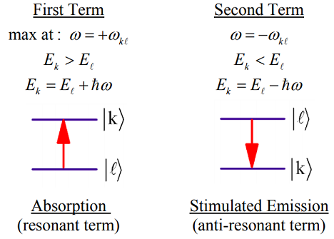
If we consider only absorption,

\[P _ {k \ell} = \left| b _ {k} \right|^{2} = \frac {\left| V _ {k l} \right|^{2}} {\hbar^{2} \left( \omega _ {k t} - \omega \right)^{2}} \quad \sin^{2} \left[ \frac {1} {2} \left( \omega _ {k \ell} - \omega \right) t \right] \label{2.163}\]

We can compare this with the exact expression:

\[P _ {k \ell} = \left| b _ {k} \right|^{2} = \frac {\left| V _ {k l} \right|^{2}} {\hbar^{2} \left( \omega _ {k t} - \omega \right)^{2} + \left| V _ {k l} \right|^{2}} \sin^{2} \left[ \frac {1} {2 \hbar} \sqrt {\left| V _ {k l} \right|^{2} + \left( \omega _ {k \ell} - \omega \right)^{2}} t \right] \label{2.164}\]

Again, we see that the first-order expression is valid for couplings \(\left| V _ {k \ell} \right|\) that are small relative to the detuning \(\Delta \omega = \left( \omega _ {k \ell} - \omega \right)\). The maximum probability for transfer is on resonance \(\omega _ {k \ell} = \omega\)

Similar to our description of the constant perturbation, the long time limit for this expression leads to a delta function \(\delta \left( \omega _ {k \ell} - \omega \right)\). In this long time limit, we can neglect interferences between the resonant and antiresonant terms. The rates of transitions between \(k\) and \(\ell\) states determined from \(w _ {k \ell} = \partial P _ {k} / \partial t\) becomes

\[w _ {k \ell} = \frac {\pi} {2 \hbar^{2}} \left| V _ {k \ell} \right|^{2} \left[ \delta \left( \omega _ {k \ell} - \omega \right) + \delta \left( \omega _ {k \ell} + \omega \right) \right] \label{2.165}\]

We can examine the limitations of this formula. When we look for the behavior on resonance, expanding the sin(x) shows us that Pk rises quadratically for short times:

\[\lim _ {\Delta \omega \rightarrow 0} P _ {k} (t) = \frac {\left| V _ {k \ell} \right|^{2}} {4 \hbar^{2}} t^{2} \label{2.166}\]

This clearly will not describe long-time behavior, but it will hold for small \(P_k\), so we require

\[t \ll \frac {2 \hbar} {V _ {k \ell}} \label{2.167}\]

At the same time, we cannot observe the system on too short a time scale. We need the field to make several oscillations for this to be considered a harmonic perturbation.

\[t > \frac {1} {\omega} \approx \frac {1} {\omega _ {k \ell}} \label{2.168}\]

These relationships imply that we require

\[V _ {k \ell} \ll \hbar \omega _ {k \ell} \label{2.169}\]

Readings

1. Cohen-Tannoudji, C.; Diu, B.; Lalöe, F., Quantum Mechanics. Wiley-Interscience: Paris, 1977; p. 1299.
2. McHale, J. L., Molecular Spectroscopy. 1st ed.; Prentice Hall: Upper Saddle River, NJ, 1999; Ch. 4.
3. Sakurai, J. J., Modern Quantum Mechanics, Revised Edition. Addison-Wesley: Reading, MA, 1994.