
6.7: Advanced Quantum Theory of Organic Molecules
- Page ID
- 22187

In recent years, great progress has been made in quantum-mechanical calculations of the properties of small organic molecules by so-called ab initio methods, which means calculations from basic physical theory using only fundamental constants, without calibration from known molecular constants. Calculations that are calibrated by one or more known properties and then used to compute other properties are called "semiempirical" calculations.
It should be made clear that there is no single, unique ab initio method. Rather, there is a multitude of approaches, all directed toward obtaining useful approximations to mathematical problems for which no solution in closed form is known or foreseeable. The calculations are formidable, because account must be taken of several factors: the attractive forces between the electrons and the nuclei, the interelectronic repulsions between individual electrons, the internuclear repulsions, and the electron spins.
The success of any given ab initio method usually is judged by how well it reproduces known molecular properties with considerable premium for use of tolerable amounts of computer time. Unfortunately, many ab initio calculations do not start from a readily visualized physical model and hence give numbers that, although agreeing well with experiment, cannot be used to enhance one's qualitative understanding of chemical bonding. To be sure, this should not be regarded as a necessary condition for making calculations. But it also must be recognized that the whole qualitative orbital and hybridization approach to chemical bonding presented in this chapter was evolved from mathematical models used as starting points for early ab initio and semiempirical calculations.
The success of any given ab initio method is judged by how well it reproduces known molecular properties.
The efforts of many chemical theorists now are being directed to making calculations that could lead to useful new qualitative concepts of bonding capable of increasing our ability to predict the properties of complex molecules. One very successful ab initio procedure, called the "generalized valence-bond" (GVB) method, avoids specific hybridization assignments for the orbitals and calculates an optimum set of orbitals to give the most stable possible electronic configuration for the specified positions of the atomic nuclei. Each chemical bond in the GVB method involves two electrons with paired spins in two more or less localized atomic orbitals, one on each atom. Thus the bonds correspond rather closely to the qualitative formulations used previously in this chapter, for example Figure 6-14.
The "generalized valence-bond" (GVB) method, avoids specific hybridization assignments for the orbitals and calculates an optimum set of orbitals to give the most stable possible electronic configuration for the specified positions of the atomic nuclei.
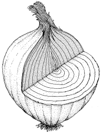
Electron-amplitude contour diagrams of the GVB orbitals for ethene are shown in Figure 6-22. Let us be clear about what these contour lines represent. They are lines of equal electron amplitude analogous to topological maps for which contour lines are equal-altitude lines. The electron amplitudes shown are those calculated in the planes containing the nuclei whose positions are shown with crosses. In general, the amplitudes decrease with distance from the nucleus. The regions of equal-electron amplitude for \(s\)-like orbitals (middle-right of Figure 6-22) surround the nuclei as a set of concentric shells corresponding to the surfaces of the layers of an onion (Figure 6-23). With the \(sp^2\)-like orbitals, the amplitude is zero at the nucleus of the atom to which the orbital belongs.

The physical significance of electron amplitude is that its square corresponds to the electron density, a matter that we will discuss further in Chapter 21. The amplitude can be either positive or negative, but its square (the electron density) is positive, and this is the physical property that can be measured by appropriate experiments.
Looking down on ethene, we see at the top of Figure 6-22 two identical \(C-C\) \(\sigma\)-bonding orbitals, one on each carbon, directed toward each other. The long dashed lines divide the space around the atom into regions of opposite orbital phase (solid is positive and dotted is negative). The contours for one of the \(C-H\) bonding orbitals are in the middle of the figure, and you will see that the orbital centered on the hydrogen is very much like an \(s\) orbital, while the one on the carbon is a hybrid orbital with considerable \(p\) character. There are three other similar sets of orbitals for the other ethene \(C-H\) bonds.
When we look at the molecule edgewise, perpendicular to the \(C-C\) \(\sigma\) bond, we see the contours of the individual, essentially \(p\)-type, orbitals for \(\pi\) bonding. Ethyne shows two sets of these orbitals, as expected.
What is the difference between the GVB orbitals and the ordinary hybrid orbitals we have discussed previously in this chapter? Consider the \(sp^2\)-like orbitals (upper part of Figure 6-22) and the \(sp^2\) hybrids shown in Figure 6-9. The important point is that the \(sp^2\) hybrid in Figure 6-9 is an atomic orbital calculated for a single electron on a single atom alone in space. The GVB orbital is much more physically realistic, because it is an orbital derived for a molecule with all of the nuclei and other electrons present. Nonetheless, the general shape of the GVB \(sp^2\)-like orbitals will be seen to correspond rather closely to the simple \(sp^2\) orbital in Figure 6-9. This should give us confidence in the qualitative use of our simple atomic-orbital models.
Contributors and Attributions
John D. Robert and Marjorie C. Caserio (1977) Basic Principles of Organic Chemistry, second edition. W. A. Benjamin, Inc. , Menlo Park, CA. ISBN 0-8053-8329-8. This content is copyrighted under the following conditions, "You are granted permission for individual, educational, research and non-commercial reproduction, distribution, display and performance of this work in any format."