9.17: Kinetic Theory of Gases- The Distribution of Molecular Speeds

Molecules in the same sample of gas may have widely varying speeds. Much the same way that raindrops rolling down a window vary in speed, even though have the same composition and are exposed to the same conditions, particles within a gas vary in speed.

In some cases, we shall find it useful to know just how popular certain speeds are—that is, we might want to know what fraction of the molecules in a sample have speeds between 0 and 400 m s^–1, or how many are going 3600 to 4000 m s^–1. Such information can be obtained from a graph showing the number of molecules within speed on one axis and number of molecules on the other axis.

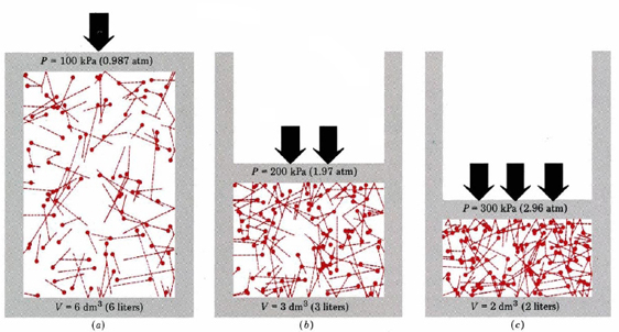
To imagine what such a graph would look like, let us study Figure 9.16.1.c in some detail. The figure depicts H₂ (g) at 300 K. Since the tails on the molecules indicate their velocities, we could count how many are traveling between 0 and 400 m s^–1, how many between 400 and 800 m s^–1, and so on. If these results are plotted as a histogram (bar graph), Figure 2a is obtained. You can see from the histogram, for example, that 20 of the 100 H₂ molecules in Figure \(\PageIndex{1}\) c are traveling between 1200 and 1600 m s^–1.

Figure \(\PageIndex{1}\) H₂ gas at 300 K.

Figure \(\PageIndex{2}\) The distribution of molecular speeds in a sample of 100 H₂ molecules at (a) 300 K and (b) 373 K. The colored line on each graph is the theoretical distribution given by the Maxwell-Boltzmann law.

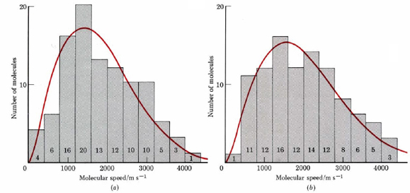
Of course any real sample of gas at 300 K and normal atmospheric pressure would contain far more than the 100 molecules in Figure 9.16.1. When the distribution of molecular speeds is measured for such a large number of molecules, the curve printed in red over the histogram is obtained. The curve is known as the Maxwell-Boltzmann distribution of molecular speeds. The most important aspect of the Maxwell-Boltzmann curve is that it is lopsided in favor of higher speeds. 

The maximum of the first curve is at 1414 m s^–1. This is the most probable speed for an H₂ molecule at 300 K. It is less than the root-mean-square velocity of 1926 m s^–1 calculated in Example 1 from Molecular Speeds. More molecules move faster than the most probable speed than move slower. Moreover, there is a small but very important fraction of molecules with very large velocities. Three have speeds between 3600 and 4000 m s^–1, and one is moving faster than 4000 m s^–1. This is about 3 times the most probable speed and more than double the average rms velocity.

Raising the temperature of a gas raises the average speed of its molecules, shifting the Maxwell-Boltzmann curve toward higher speeds, as shown in Figure \(\PageIndex{2}\) b. Increasing the temperature from 300 to 373 K increases the most probable speed from 1414 to 1577 m s^–1 and the rms velocity from 1926 to 2157 m s^–1, both increases of 11 percent.

The number of really fast molecules goes up much more significantly, however. In the range 3600 to 4000 m s^–1 the number of molecules increases from 3 to 5 (67 percent), and in the range 4000 to 4400 m s^–1, the number increases from 1 to 3 (300 percent). If we apply the Maxwell-Boltzmann distribution to 1 mole H₂(g) (instead of the 100 molecules in Figure \(\PageIndex{2}\) ), we find 0.75 million molecules moving faster than 10 000 m s^–1 at 300 K. At 373 K this number has increased to 465 million—more than 60 000 percent.

There are many things in nature which depend on the average (rms) velocity of molecules. A mercury thermometer is one, and the pressure of a gas is another. Many other things, however, are influenced by the number of very fast molecules rather than by the average velocity. One example is the human finger—in a sample of H₂(g) at 300 K it feels pleasantly warm, but at 373 K it will blister. This important difference in behavior is not caused by an 11-percent increase in the average velocity of the molecules. It is caused by a dramatic increase in the number of very energetic molecules, which occurs when the temperature is raised from 300 to 373 K. 

The rates of chemical reactions respond to the number of really fast molecules instead of the average molecular velocity, just as your finger would. Most chemical reactions can be speeded up tremendously by raising the temperature, and this is why chemists so often boil things in flasks to get reactions to occur.