8.10.9D: Ionic migration

Last updated
Save as PDF

Page ID: 20112

\( \newcommand{\vecs}[1]{\overset { \scriptstyle \rightharpoonup} {\mathbf{#1}} } \) \( \newcommand{\vecd}[1]{\overset{-\!-\!\rightharpoonup}{\vphantom{a}\smash {#1}}} \)\(\newcommand{\id}{\mathrm{id}}\) \( \newcommand{\Span}{\mathrm{span}}\) \( \newcommand{\kernel}{\mathrm{null}\,}\) \( \newcommand{\range}{\mathrm{range}\,}\) \( \newcommand{\RealPart}{\mathrm{Re}}\) \( \newcommand{\ImaginaryPart}{\mathrm{Im}}\) \( \newcommand{\Argument}{\mathrm{Arg}}\) \( \newcommand{\norm}[1]{\| #1 \|}\) \( \newcommand{\inner}[2]{\langle #1, #2 \rangle}\) \( \newcommand{\Span}{\mathrm{span}}\) \(\newcommand{\id}{\mathrm{id}}\) \( \newcommand{\Span}{\mathrm{span}}\) \( \newcommand{\kernel}{\mathrm{null}\,}\) \( \newcommand{\range}{\mathrm{range}\,}\) \( \newcommand{\RealPart}{\mathrm{Re}}\) \( \newcommand{\ImaginaryPart}{\mathrm{Im}}\) \( \newcommand{\Argument}{\mathrm{Arg}}\) \( \newcommand{\norm}[1]{\| #1 \|}\) \( \newcommand{\inner}[2]{\langle #1, #2 \rangle}\) \( \newcommand{\Span}{\mathrm{span}}\)\(\newcommand{\AA}{\unicode[.8,0]{x212B}}\)

The motion of ions in solution is mainly random

The conductance of an electrolytic solution results from the movement of the ions it contains as they migrate toward the appropriate electrodes. But the picture we tend to have in our minds of these ions moving in a orderly, direct march toward an electrode is wildly mistaken. The thermally-induced random motions of molecules is known as diffusion. The term migration refers specifically to the movement of ions due to an externally-applied electrostatic field.

The average thermal energy at temperatures within water's liquid range (given by RT ) is sufficiently large to dominate the movement of ions even in the presence of an applied electric field. This means that the ions, together with the water molecules surrounding them, are engaged in a wild dance as they are buffeted about by thermal motions (which include Brownian motion).

If we now apply an external electric field to the solution, the chaotic motion of each ion is supplemented by an occasional jump in the direction dictated by the interaction between the ionic charge and the field. But this is really a surprisingly tiny effect:

It can be shown that in a typical electric field of 1 volt/cm, a given ion will experience only about one field-directed (non-random) jump for every 10⁵ random jumps. This translates into an average migration velocity of roughly 10^–7 m sec^–1 (10^–4 mm sec^–1). Given that the radius of the H₂O molecule is close to 10^–10 m, it follows that about 1000 such jumps are required to advance beyond a single solvent molecule!

The ions migrate Independently

All ionic solutions contain at least two kinds of ions (a cation and an anion), but may contain others as well. In the late 1870's, the physicist Friedrich Kohlrausch noticed that the limiting equivalent conductivities of salts that share a common ion exhibit constant differences.

electrolyte	Λ₀(25°C)	difference	electrolyte	Λ₀ (25°C)	difference
KCl LiCl	149.9 115.0	34.9	HCl HNO₃	426.2 421.1	4.9
KNO₃ LiNO₃	145.0 140.1	34.9	LiCl LiNO₃	115.0 110.1	4.9

These differences represent the differences in the conductivities of the ions that are not shared between the two salts. The fact that these differences are identical for two pairs of salts such as KCl/LiCl and KNO₃ /LiNO₃ tells us that the mobilities of the non-common ions K⁺ and LI⁺ are not affected by the accompanying anions.

Kohlrausch's law greatly simplifies estimates of Λ₀

This principle is known as Kohlrausch's law of independent migration, which states that in the limit of infinite dilution,

Each ionic species makes a contribution to the conductivity of the solution that depends only on the nature of that particular ion, and is independent of the other ions present.

Kohlrausch's law can be expressed as

Λ₀ = Σ λ⁰₊ + Σ λ⁰_–

This means that we can assign a limiting equivalent conductivity λ₀ to each kind of ion:

Limiting ionic equivalent conductivities at 25°C, S cm^–1 eq^–1
cation	H₃O⁺	NH₄⁺	K⁺	Ba²⁺	Ag⁺	Ca²⁺	Sr²⁺	Mg²⁺	Na⁺	Li⁺
λ₀	349.98	73.57	73.49	63.61	61.87	59.47	59.43	53.93	50.89	38.66
anion	OH^–	SO₄^2–	Br^–	I^–	Cl^–	NO_3^–	ClO_3^–	CH₃COO^–	C₂H₅COO^–	C₃H₇COO^–
λ₀	197.60	80.71	78.41	76.86	76.30	71.80	67.29	40.83	35.79	32.57

Just as a compact table of thermodynamic data enables us to predict the chemical properties of a very large number of compounds, this compilation of equivalent conductivities of twenty different species yields reliable estimates of the of Λ₀ values for five times that number of salts.

We can now estimate weak electrolyte limiting conductivities

One useful application of Kohlrausch's law is to estimate the limiting equivalent conductivities of weak electrolytes which, as we observed above, cannot be found by extrapolation. Thus for acetic acid CH₃COOH ("HAc"), we combine the λ₀ values for H₃O⁺ and CH₃COO^– given in the above table:

Λ_⁰HAc = λ⁰_H+ + λ⁰_Ac–

How fast do ions migrate in solution?

Movement of a migrating ion through the solution is brought about by a force exerted by the applied electric field. This force is proportional to the field strength and to the ionic charge. Calculations of the frictional drag are based on the premise that the ions are spherical (not always true) and the medium is continuous (never true) as opposed to being composed of discrete molecules. Nevertheless, the results generally seem to be realistic enough to be useful.

According to Newton's law, a constant force exerted on a particle will accelerate it, causing it to move faster and faster unless it is restrained by an opposing force. In the case of electrolytic conductance, the opposing force is frictional drag as the ion makes its way through the medium. The magnitude of this force depends on the radius of the ion and its primary hydration shell, and on the viscosity of the solution.

Eventually these two forces come into balance and the ion assumes a constant average velocity which is reflected in the values of λ₀ tabulated in the table above.

The relation between λ₀ and the velocity (known as the ionic mobility μ₀) is easily derived, but we will skip the details here, and simply present the results:

Anions are conventionally assigned negative μ₀ values because they move in opposite directions to the cations; the values shown here are absolute values |μ₀|. Note also that the units are cm/sec per volt/cm, hence the cm² term.

Absolute limiting mobilities of ions at 25°C, (cm² volt^–1 sec^–1) × 100
cation	H₃O⁺	NH₄⁺	K⁺	Ba²⁺	Ag⁺	Ca²⁺	Sr²⁺	Mg²⁺	Na⁺	Li⁺
μ₀	0.362	0.0762	0.0762	0.0659	0.0642	0.0616	0.0616	0.0550	0.0520	0.0388
anion	OH^–	SO₄^2–	Br^–	I^–	Cl^–	NO_3^–	ClO_3^–	CH₃COO^–	C₂H₅COO^–	C₃H₇COO^–
μ₀	.2050	0.0827	0.0812	0.0796	0.0791	0.0740	0.0705	0.0461	0.0424	0.0411

As with the limiting conductivities, the trends in the mobilities can be roughly correlated with the charge and size of the ion. (Recall that negative ions tend to be larger than positive ions.)

Cations and anions carry different fractions of the current

In electrolytic conduction, ions having different charge signs move in opposite directions. Conductivity measurements give only the sum of the positive and negative ionic conductivities according to Kohlrausch's law, but they do not reveal how much of the charge is carried by each kind of ion. Unless their mobilities are the same, cations and anions do not contribute equally to the total electric current flowing through the cell.

Recall that an electric current is defined as a flow of electric charges; the current in amperes is the number of coulombs of charge moving through the cell per second. Because ionic solutions contain equal quantities of positive and negative charges, it follows that the current passing through the cell consists of positive charges moving toward the cathode, and negative charges moving toward the anode. But owing to mobility differences, cations and ions do not usually carry identical fractions of the charge.

Transference numbers are often referred to as transport numbers; either term is acceptable in the context of electrochemistry. The fraction of charge carried by a given kind of ion is known as the transference number \(t_{\pm}\). For a solution of a simple binary salt,

\[ t_+ = \dfrac{\lambda_+}}{\lambda_+ + \lambda_-}\]

and

\[ t_- = \dfrac{\lambda_-}}{\lambda_+ + \lambda_-}\]

By definition,

\[t_+ + t_– = 1.\]

To help you visualize the effects of non-identical transference numbers, consider a solution of M⁺ X^– in which t₊ = 0.75 and t_– = 0.25. Let the cell be divided into three [imaginary] sections as we examine the distribution of cations and anions at three different stages of current flow.

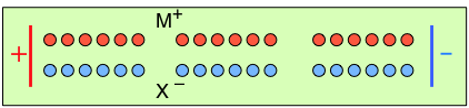	Initially, the concentrations of M⁺ and X^– are the same in all parts of the cell.
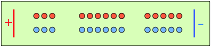
	After 4 faradays of charge have passed through the cell, 3 eq of cations and 1 eq of anions have crossed any given plane parallel to the electrodes. Note that 3 anions are discharged at the anode, exactly balancing the number of cations discharged at the cathode.
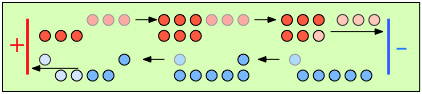
	In the absence of diffusion, the ratio of the ionic concentrations near the electrodes equals the ratio of their transport numbers.

Transference numbers can be determined experimentally by observing the movement of the boundary between electrolyte solutions having an ion in common, such as LiCl and KCl:

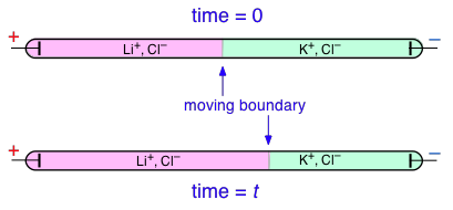
In this example, K⁺ has a higher transference number than Li⁺, but don't try to understand why the KCl boundary move to the left; the details of how this works are rather complicated and not important for the purposes of this this course.

H⁺ and OH^– ions "migrate" without moving, and rapidly!

You may have noticed from the tables above that the hydrogen- and hydroxide ions have extraordinarily high equivalent conductivities and mobilities. This is a consequence of the fact that unlike other ions which need to bump and nudge their way through the network of hydrogen-bonded water molecules, these ions are participants in this network. By simply changing the H₂O partners they hydrogen-bond with, they can migrate "virtually". In effect, what migrates is the hydrogen-bonds, rather than the physical masses of the ions themselves.

This process is known as the Grothuss Mechanism. The shifting of the hydrogen bonds occurs when the rapid thermal motions of adjacent molecules brings a particular pair into a more favorable configuration for hydrogen bonding within the local molecular network. Bear in mind that what we refer to as "hydrogen ions" H⁺(aq) are really hydronium ions H₃O⁺. It has been proposed that the larger aggregates H₅O₂⁺and H₉O₄⁺ are important intermediates in this process.

It is remarkable that this virtual migration process was proposed by Theodor Grotthuss in 1805 — just five years after the discovery of electrolysis, and he didn't even know the correct formula for water; he thought its structure was H–O–O–H.

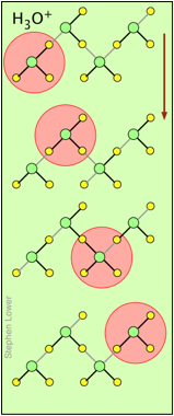
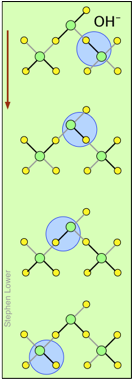
These two diagrams will help you visualize the process. The successive downward rows show the first few "hops" made by the virtual H⁺ and OH^–ions as they move in opposite directions toward the appropriate electrodes. (Of course, the same mechanism is operative in the absence of an external electric field, in which case all of the hops will be in random directions.)

Covalent bonds are represented by black lines, and hydrogen bonds by gray lines.