Convolution-Based Smoothing

Overview

Digital filtering is a data treatment method that enhances the signal-to-noise ratio of an analytical signal through the convolution of a data set with an appropriate filter. This treatment method is another smoothing technique. If the filter is unweighted, it will perform in a similar manner to the boxcar filter. That is, it filters out rapidly changing signals by averaging over a relatively long time but has a negligible effect on slowly changing signals, and it too behaves as a software-based low-pass filter. However, a weighted filter may be constructed to mimic a low-pass, high-pass or even a bandpass filter. This module will focus on a weighted filter application based on least-squares quadratic smoothing that was popularized by Savitzky and Golay in the 1960’s.

Convolution

Before we explore the differences in the meaning and construction of unweighted versus weighted filters, the concept of convolution needs to be addressed. Let’s start with an analytical signal sampled every second for ten seconds. The raw data in this ideal case, which is represented in the figure below, consists of a slowly changing peak-shaped function.

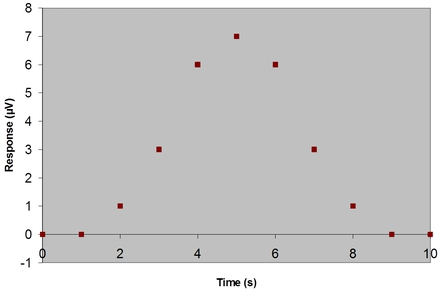
For the moment, let’s ignore the independent variable (i.e. x-axis) and treat this instrumental response as a vector. We can represent the data above by the following matrix:

x = [ 0 0 1 3 6 7 6 3 1 0 0 ]

and a three-point unweighted filter to convolve the raw data

f = [ 1 1 1 ]

The result will be a smoothed data matrix, x’

The convolution process involves the following steps:

1. Matrix multiplication of the first raw data segment with the same number of array elements as the appropriate filter function, f. The filter function has the same sampling rate as the raw data.
   1. This operation is called the dot product.

      \[\mathrm{f\cdot x = \sum\limits_{i = 1}^{n}f_ix_i \:\:\:(n = length\: of\: filter)}\]

   2. So for the first set of three raw data points:

      \[\mathrm{f\cdot x=[f_1\:\:\: f_2\:\:\: f_3] \cdot
      \begin{bmatrix}\ce x_1
      \\ \ce x_2
      \\ \ce x_3
      \end{bmatrix} =(f_1x_1 + f_2x_2 + f_3x_3)}\]

2. Normalizing the dot product with the sum of the filter elements and placing the result in the smooth data matrix with an x-value equivalent to the x-value of the center of the filter function.

   \[\mathrm{x'_2 = \dfrac{f \cdot x}{\sum\limits_{i = 1}^{n}f_i}= \dfrac{(f_1x_1 + f_2x_2 + f_3x_3)}{(f_1 + f_2 + f_3)}}\]

   1. So in this case, x’₂ has the same time as x₂ (i.e. time = 2 s).
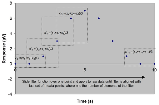
3. Slide the filter function over one data point and repeat the matrix multiplication process, placing the next normalized dot product as the next array element in the smoothed data matrix. Therefore,

   \[\mathrm{x'_3 = \dfrac{f \cdot x}{\sum\limits_{i = 1}^{n}f_i}
   = \dfrac{\sum\limits_{i = 1}^{n}f_ix_{(i+1)}}{\sum\limits_{i = 1}^{n}f_i}
   = \dfrac{(f_1x_2 + f_2x_3 + f_3x_4)}{(f_1 + f_2 + f_3)}}\]

   1. x’₃ has the same time as x₃ (i.e. time = 3 s).
4. Repeat step 3 until the leading edge of the filter has the same x-value as the last point in the raw data matrix. This means that (n-1)/2 data points will be lost from each side of x’

Because the filter function is unweighted, we call this convolution process the moving window averaging technique, as shown in the figure below.

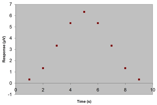
Convolving the filter function with the original response in the previous figure results in the smoothed response below.

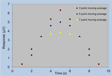
Effect of Unweighted Filter Width

In the unweighted moving window averaging approach, we assume that each data point is equally important in the instrumental response above. This works well if the peak width is much larger than the filter width. However, if the width of the filter is comparable to the peak width of the signal, applying an unweighted filter distorts the signal, decreasing the signal intensity and increasing its width. In the figure below, the raw data is smoothed by a 3-point, 5-point, and 7-point unweighted filter.

Weighted (Savitzky-Golay) Filters

In order to avoid distorting the signal significantly, one convolves the raw data with a filter that looks more like the signal itself. A weighted filter that emphasizes the response at the central filter element and de-emphasizes the response at the outer filter elements is used. This approach, which is called least-squares polynomial smoothing, was popularized in analytical chemistry by Savitzky and Golay. Savitzky and Golay used the least-squares approach to derive a set of convolution integers for a given filter width. Below is a list of Savitzky-Golay coefficients for 5, 9, and 13-point quadratic smoothing of instrumental responses.

Filter Points	13	9	5
-6	-11
-5	0
-4	9	-21
-3	16	14
-2	21	39	-3
-1	24	54	12
0	25	59	17
1	24	54	12
2	21	39	-3
3	16	14
4	9	-21
5	0
6	-11
Normalizing Factor	143	231	35

If we use a five-point filter function, instead of the unweighted function below

f = [ 1 1 1 1 1 ]

we would use the Savitzky-Golay coefficients

f = [ -3 12 17 12 -3 ]

using the original raw data, the normalized dot product for the first smoothed data point would be

\[\mathrm{x'_3 = \dfrac{f \cdot x}{\sum\limits_{i = 1}^{n}f_i} = \dfrac{(f_1x_1 + f_2x_2 + f_3x_3 + f_4x_4 + f_5x_5)}{(f_1 + f_2 + f_3 + f_4 + f_5)}\\
= \dfrac{((-3*0)+(12*0)+(17*1)+(12*3)+(-3*6))}{((-3)+12+17+12+(-3))}}\]

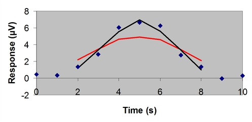
Just like the unweighted moving average smooth, the raw data would be convolved with the weighted moving average smooth using the appropriate Savitzky-Golay coefficients. A comparison of the 5-point unweighted and weighted moving average smoothing functions on a "noisy" version of the raw data set is shown below. Notice that the polynomial filter (smoothed response in black) distorts the signal to a lesser extent than the unweighted filter (smoothed response in red).

Points to Consider Using Moving Average Filtering

• The moving average technique retains greater data density than boxcar averaging.
• The moving average technique is straightforward to implement.
• Improvement in S/N is proportional to (# filter elements)^1/2 if the noise is normally distributed.
• (N-1)/2 points are lost on either end of the smoothed data set, where N is the filter length.
• Significant distortion and loss of resolution may occur if the length of the filter is comparable to the peak width. It is best to implement a moving average with a filter width much smaller than the narrowest peak to be smoothed.
• Optimal filter choices are typically chosen in an empirical fashion.

Click here to work on a moving average exercise