Answers

Last updated
Save as PDF

Page ID: 76366

Alexander Scheeline & Thomas M. Spudich
Analytical Sciences Digital Library

\( \newcommand{\vecs}[1]{\overset { \scriptstyle \rightharpoonup} {\mathbf{#1}} } \) \( \newcommand{\vecd}[1]{\overset{-\!-\!\rightharpoonup}{\vphantom{a}\smash {#1}}} \)\(\newcommand{\id}{\mathrm{id}}\) \( \newcommand{\Span}{\mathrm{span}}\) \( \newcommand{\kernel}{\mathrm{null}\,}\) \( \newcommand{\range}{\mathrm{range}\,}\) \( \newcommand{\RealPart}{\mathrm{Re}}\) \( \newcommand{\ImaginaryPart}{\mathrm{Im}}\) \( \newcommand{\Argument}{\mathrm{Arg}}\) \( \newcommand{\norm}[1]{\| #1 \|}\) \( \newcommand{\inner}[2]{\langle #1, #2 \rangle}\) \( \newcommand{\Span}{\mathrm{span}}\) \(\newcommand{\id}{\mathrm{id}}\) \( \newcommand{\Span}{\mathrm{span}}\) \( \newcommand{\kernel}{\mathrm{null}\,}\) \( \newcommand{\range}{\mathrm{range}\,}\) \( \newcommand{\RealPart}{\mathrm{Re}}\) \( \newcommand{\ImaginaryPart}{\mathrm{Im}}\) \( \newcommand{\Argument}{\mathrm{Arg}}\) \( \newcommand{\norm}[1]{\| #1 \|}\) \( \newcommand{\inner}[2]{\langle #1, #2 \rangle}\) \( \newcommand{\Span}{\mathrm{span}}\)\(\newcommand{\AA}{\unicode[.8,0]{x212B}}\)

Blank Subtraction

The signal at 588.9 nm = 43756 counts, a combination of signal and background. The signal at 589.1 nm = 1210 counts, all background. Thus the 588.9 nm signal is 43756-1210 = 42546 counts above background and the sensitivity of the measurement is 42546 counts/100 ppb or 425.5 counts/ppb. Thus a 10 ppb sample should have a total signal of 10*425.5 = 4255 counts (signal) + 1210 counts (background) = 5465 counts. If we hadn't measured background, the sensitivity would have seemed to be 43756/100 = 437.6 counts/ppb, and 5465 counts/(437.6 counts/ppb) gives 12.5 ppb, at 25% overestimation.
Now the signal at 588.9 nm is on top of a smaller background than we previously computed because the signal at 589.1 nm includes 1% stray light from the 588.9 nm data. Thus 438 counts of the signal at the longer wavelength is from stray light and the true background is 1210-438 = 772 counts. The signal due to sodium at the shorter wavelength is 43756-772 = 42984 counts. 10 ppb then will generate 4298 counts from sodium plus 772 counts from background or 5070 counts. If we had completely ignored background, the apparent concentration of the 10 ppb solution would be 5070/43756*100 ppb = 11.6 ppb, still a 16% error, but less than before. Note that the measurement of stray light has to be done using an emission line much narrower than the resolution of the instrument so that we can be sure that we're not looking at the wings of the emission line. It is tricky to determine the difference between plasma background and proportionate/stray light background.
4.01% - 0.02% = 3.99%. We have no information on the precision of any of the numbers, so we have no idea how many of the figures are significant.

Problems for Curve Fitting Strategies

Plotting the data, the working curve looks linear to the unaided eye. Doing a linear regression, one finds
Signal = (169±9) + (1199±7) C.
Quadratic regression gives
Signal = (149±4) + (1258±8) C - (24±3)C²

Inspection of the equations generates no insight. Here are residual plots for the data:

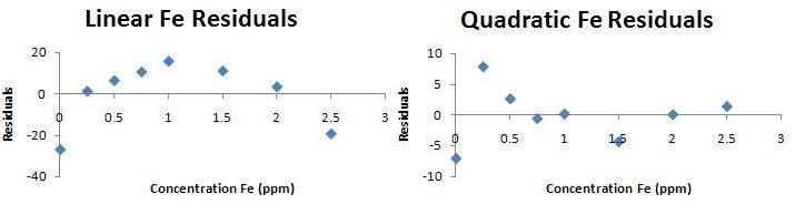
There's a pattern to the residuals for the linear fit, while the residuals are random for the quadratic fit. The quadratic curve is preferred. Useful working range for the linear curve is 0.25 ppm to 2 ppm. Useful range for the quadratic curve is only DEMONSTRATED from 0.5 ppm to 2.5 ppm. It is likely we could work at higher concentration, but one of the easily avoided errors in any analytical method is working outside the range over which one has validated calibration data.
Take the ratio of Ca emission/Y emission and plot vs. [Ca²⁺]. The resulting working curve is I_Ca/I_Y=(0.7430±0.0009) + (1.2491±0.0015) C_Ca. The first "gotcha" in the analysis of the unknown is that there's only 39 mL of Y-containing solution, not 40, so the Y raw intensity needs to be scaled up by 40/39 from the raw value to be able to use the original working curve. Thus, in computing the intensity ratio, use I_Y = 3315*40/39 = 3400. Now we find C_Ca= (4988/3400 - 0.7430)/1.2491 = 0.580 ppm. But that's the concentration aspirated into the ICP. What we care about is the concentration in the blood serum. Since we diluted 1 mL of serum into 100 mL before determination, the actual concentration in serum is 58.0 ppm. Take the ratio of Ca emission/Y emission and plot vs. [Ca²⁺]. The resulting working curve is I_Ca/I_Y=(0.7430±0.0009) + (1.2491±0.0015) C_Ca. The first "gotcha" in the analysis of the unknown is that there's only 39 mL of Y-containing solution, not 40, so the Y raw intensity needs to be scaled up by 40/39 from the raw value to be able to use the original working curve. Thus, in computing the intensity ratio, use I_Y = 3315*40/39 = 3400. Now we find C_Ca= (4988/3400 - 0.7430)/1.2491 = 0.580 ppm. But that's the concentration aspirated into the ICP. What we care about is the concentration in the blood serum. Since we diluted 1 mL of serum into 100 mL before determination, the actual concentration in serum is 58.0 ppm.

Time Gating

If the rotation rate is H, the beam sweeps out a distance of 2πDH each second. If the mirror rotates through an angle θ, the reflected image rotates through 2θ, since the angle of incidence equals the angle of reflection. Given the pixel width p, the time the beam is on a given pixel is p/2πDH. Rule of thumb is that data must be separated by 3 pixels to ensure distinctiveness, so the useful time resolution is 3p/2πDH. For a 25 µm pixel CCD, 1 m focal length, 60 revolutions per second (i.e. the mirror is driven by a synchronous AC motor on the North American power grid), the time resolution = 3*2.5×10^-5 m/(2π*1 m * 60 s^-1) = 0.2 µs. Note that one may readily spin a mirror at higher speeds, and one may also use smaller pixels. At 1 KHz (the mechanical stresses make this a fairly high speed, at least in air) and with 6 µm pixels, the time resolution improves to 3 ns.