a) Chronoamperometry

Consider a situation where a solid electrode is immersed in a solution containing the oxidized form (Ox) of a redox couple at some known initial concentration (C₀), say 1.0 mM. Initially the electrode is poised at a potential (E_i) well positive of the E⁰’ for the Red/Ox couple, assuring that only Ox is present in the solution. The solution also contains an excess of some inert electrolyte, and you are working in a still environment to assure that flux to the electrode is strictly diffusion controlled. At a time designated t₀, the potential is stepped to a value significantly more negative than the E⁰’ for the redox couple (E_s), and Ox in the vicinity of the electrode is immediately converted (assuming reversible kinetics) to Red.

As a consequence of the conversion, the concentration of Ox directly adjacent to the electrode is reduced to zero from its initial, bulk concentration of 1.0 mM. This leads to the formation of a concentration gradient for Ox, through which Ox from the bulk of solution must diffuse to the electrode surface, where it is immediately reduced to Red. The longer the electrode remains at this reducing potential, the further away from the electrode the region depleted of Ox, called the diffusion layer, extends. A similar, but opposite gradient exists for Red, which after formation is free to diffuse away from the electrode surface, reaching further into the bulk as time passes. This situation is summarized in Figure 10.

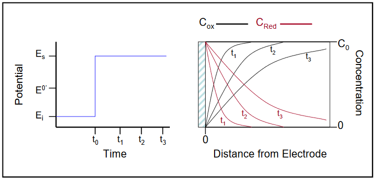
Figure 10

As discussed in the previous section, the faradaic current under diffusion controlled conditions is related directly to the concentration gradient, ∂C_i / ∂x, evaluated at x = 0. Thus, as the slope of the concentration profile for Ox decreases with time following the potential step, so will the observed current. In the example above, the concentration of Ox at the surface was driven immediately to zero for a step to a potential well negative of the E⁰’ for the couple. In general for a reversible system (reduction), the ratio of [Red] to [Ox] at the surface is given by the Nernst equation at any potential, with the ratio reaching 100:1 at a value 118 mV more negative than the E⁰’. Additional information on the formation of concentration gradients, and an excellent Applet demonstrating the potential step experiment can be found at http://www.chem.uoa.gr/applets/Apple...l_Diffus2.html.⁶

Chronoamperometry experiments are most commonly either single potential step, in which only the current resulting from the forward step as described above is recorded, or double potential step, in which the potential is returned to a final value (E_f) following a time period, usually designated as τ, at the step potential (E_s).

The most useful equation in chronoamperometry is the Cottrell equation, which describes the observed current (planar electrode) at any time following a large forward potential step in a reversible redox reaction (or to large overpotential) as a function of t^-1/2.

\[\mathrm{i_t = \dfrac{n\, F\, A\, C_0\, D_0^{1/2}}{π^{1/2}\, t^{1 / 2}}}\]

where

n = stoichiometric number of electrons involved in the reaction; F = Faraday’s constant (96,485 C/equivalent), A = electrode area (cm²), C₀ = concentration of electroactive species (mol/cm³), and D₀ = diffusion constant for electroactive species (cm²/s).

The current due to double layer charging, described in a previous section, also contributes to the total seen following a potential step. By nature however, this capacitive current, i_C, decays as a function of 1/t and is only significant during the initial period (generally a few ms) following the step. It can be easily recorded by performing the experiment in a cell containing only electrolyte, and digitally subtracted. Usually it can be avoided altogether by only considering i-t data taken during the last 90% of the step time.

Double potential step chronoamperometry is illustrated in Figure 11. The potential step program is shown at left, with a forward potential step from E_i to E_s of duration τ. The reverse potential step shown is to a final potential, E_f, of E_f = E_i, though other values of E_f may be desirable in some experiments. In general, the current on the reverse step is also recorded for a time equal to τ. As expected from the Cottrell equation, the observed current for the forward step decays as t^-1/2. In this example, the electron transfer is both chemically and electro-chemically reversible. The reverse current-time trace is conceptually more difficult to describe than that for the forward step. Those interested are referred to the treatment found in Bard and Faulkner.² An uncomplicated, reversible system can be identified by comparing the reverse and forward current values measured at the same time interval following each respective potential step. For example, the current values measured at a time equal to τ/2 after each step (designated i_r and i_f in the previous figure) for such a system would yield a value equal to 0.293 for the ratio of [-i_r (2τ) / i_f (τ)]. The presence of chemical reaction(s) following electron transfer will generally result in ratios that deviate from this theoretical value.

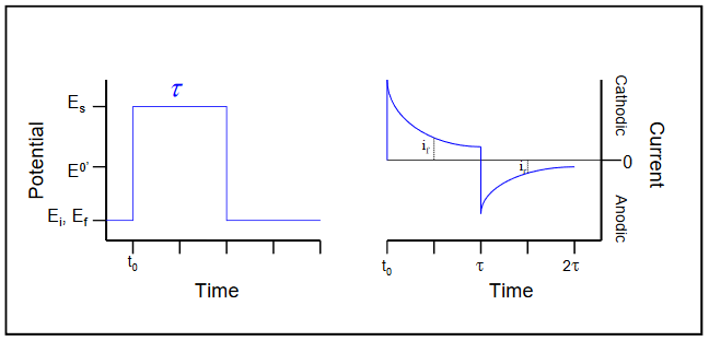
Figure 11

Chronoamperometry lends itself well to the accurate measurement of electrode area (A) by use of a well-defined redox couple (known n, C₀, and D₀). With a known electrode area, measurement of either n or D₀ for an electroactive species is easily accomplished. The double potential step method is often applied in the measurement of rate constants for chemical reactions (including product adsorption) occurring following the forward potential step next section.