Part IV: Ways to Model Data

Investigation 18.

So, what does it mean to build a model? Consider the histograms in Figure 4. What property of the population are we attempting to model? What do your responses imply about the model’s general mathematical form? What does it mean to test a model and how might we accomplish this?

For the histograms in Figure 4, we wish to model the number of each color of M&M in a 1.69-oz bag of plain M&Ms. A suitable mathematical model will need to predict the probability, p, of drawing X M&Ms of a particular color when we select a sample of N M&Ms from the population of all M&Ms; thus, we expect the equation to be a function of the form P = f(X,N).

To test a model, we need to compare the results predicted by our model to the results of our experiments. For example, Table 2 contains results for the distribution of colors and the net weight of plain M&Ms in 1.69-oz bags. If we develop a model that predicts successfully the average number of yellow M&Ms in a 1.69-oz bag, then we have some confidence that the model is reasonable. Of course, we need to define how we decide if a model’s predictions agree with our data, which we will explore in greater detail in Part V.

Investigation 19.

The box and whisker plot in Figure 1 includes data from the analysis of 30 samples of 1.69-oz bags of plain M&Ms. Collectively, the samples have 1699 M&Ms, of which 435 are yellow. If you pick one M&M at random from these 1699 M&Ms, what is the probability, p, that it is yellow? Suppose that this probability applies to the population of all plain M&Ms. If we draw a sample of five M&Ms from this population, what is the probability that the sample contains no yellow M&Ms? Repeat for each of 1–5 yellow M&Ms. Construct a histogram of your results and report the mean and the variance. Repeat this analysis for green M&Ms. Compare your two histograms and discuss their similarities and their differences. Using the data in Table 2, comment on the suitability of the binomial distribution for modeling the number of yellow M&Ms in samples of five M&Ms.

Given the data from our samples, the probability of selecting a single yellow M&M is

\[p=\dfrac{435}{1699} =0.256\]

If we assume that this probability applies to the population of plain M&Ms and if we assume a binomial distribution, then the probability of drawing zero yellow M&Ms in a sample of five M&Ms is

\[P(0,5)= \dfrac{5!}{0! (5 -0 )!} × (0.256)^0 ×(1 -0.256)^{5 -0} =0.228\]

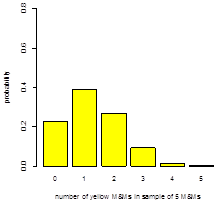
The remaining probabilities are 0.392, 0.270, 0.093, 0.016, and 0.001 for P(1, 5) to P(5, 5), respectively; the resulting distribution is shown below on the left. The mean and the variance are

\[μ=Np=5×0.256=1.28\]

\[σ^2 =Np(1-p)=5×0.256×(1-0.256)=0.95\]

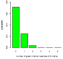
For green M&Ms, there are 110 in the combined sample of 1699 plain M&Ms, or a probability of 0.0647. The probabilities for drawing zero to five green M&Ms in a sample of five M&Ms are, respectively, 0.716, 0.248, 0.034, 0.002, 0.000, and 0.000; the resulting histogram is shown above to the right. The mean and the variance are 0.32 and 0.30, respectively.

In terms of similarities, both histograms encompass a net probability of 1.00 as they span the six possible outcomes when drawing a sample of five M&Ms, and neither histogram is symmetrical around its most probable outcome. The most importance difference between the two histograms is the relative frequencies of the possible outcomes; in particular, a sample of five M&Ms is more than 3× as likely to have no green M&Ms than to have no yellow M&Ms, and is more than 3× as likely to have three or more yellow M&Ms than three or more green M&Ms. Given their relative abundances—25.6% of the 1699 total M&Ms are yellow versus just 6.47% for green—these differences make sense.

From Table 2, we know that actual distribution of results for yellow M&Ms in the first five sampled is seven with no yellow M&Ms, 13 with one yellow M&M, eight with two yellow M&Ms, two with three yellow M&Ms, and zero with four and with five yellow M&Ms. The following table compares the results of our experiment and the predicted results from our model.

P(X,N)	experiment	model	absolute error
P(0,5)	0.233	0.228	0.005
P(1,5)	0.433	0.392	0.041
P(2,5)	0.267	0.270	–0.003
P(3,5)	0.067	0.093	–0.026
P(4,5)	0.000	0.016	–0.016
P(5,5)	0.000	0.001	–0.001

As one sample is 1/30th, or 0.033, of the 30 samples, the absolute errors represent an oversampling of approximately one for P(1,5) and an undersampling of approximately one for P(3,5), an experimental uncertainty that seems reasonable given the relatively small number of samples and the relatively small value for N.

Investigation 20.

Explain why we cannot use the binomial distribution to model the distribution of yellow M&Ms in 1.69-oz bags of plain M&Ms.

The binomial distribution predicts the probability of a particular event, X, such as drawing five yellow M&Ms, in samples of fixed size, N, where X ≤ N. Because the number of M&Ms varies from bag-to-bag, the value of N varies from bag-to-bag and we cannot model the distribution of M&Ms in 1.69-oz bags of plain M&Ms; we could, however, model the distribution of yellow M&Ms in all 1.69-oz bags that contain the same total number of M&Ms.

Investigation 21.

The histograms in Figure 4 include data from the analysis of 30 samples of 1.69-oz bags of plain M&Ms. Collectively, the samples have an average of 14.5 yellow M&Ms per bag. Suppose this rate applies to the population of all 1.69-oz bags of plain M&Ms. If you pick a 1.69-oz bag of plain M&Ms at random, what is the probability that it contains exactly 11 yellow M&Ms? Repeat for each of 0–29 yellow M&Ms. Construct a histogram that shows the actual distribution of bags of M&Ms for each of 0–29 yellow M&Ms, using a bin size of 1 unit, and overlay a line plot that shows the predicted distribution of bags; be sure to you use the same scale for each plot’s y-axis. Comment on your results.

If we assume that the average rate of 14.5 yellow M&Ms per bag applies to the population of plain M&Ms, and assume a Poisson distribution, then the probability of finding 11 yellow M&Ms in a 1.69-oz package of plain M&Ms is

\[P(11,14.5)=\dfrac{e^{-14.5}14.5^0}{11!}=0.0753\]

or 2.3 out of 30 bags of M&Ms. The actual number of bags of M&Ms that contain each of 0–29 yellow M&Ms and the predicted probabilities are gathered in the following table; the predicated probabilities from the Poisson equation are multiplied by 30 so that the two results are on the same scale.

X	Actual	P(X,14.5)
0	0	0.000
1	0	0.000
2	0	0.002
3	0	0.008
4	0	0.028
5	1	0.081
6	0	0.195
7	1	0.405
8	3	0.733
9	0	1.181
10	1	1.713
11	0	2.258
12	1	2.729
13	3	3.043
14	4	3.152
15	3	3.047
16	5	2.761
17	2	2.355
18	2	1.897
19	1	1.448
20	0	1.050
21	0	0.725
22	1	0.478
23	2	0.301
24	0	0.182
25	0	0.106
26	0	0.059
27	0	0.032
28	0	0.016
29	0	0.008

The resulting histogram for the actual distribution of yellow M&Ms in the 30 samples and the predicted distribution are shown here

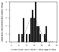
Two factors make difficult any comparison of the actual counts to the predicted counts: the actual counts are discrete (we can have 0 or 1 bag with five yellow M&Ms, but we cannot have 0.08 bags with five yellow M&Ms), and the number of samples, at 30, is too small to allow for predicted counts of at least one bag for outcomes with a small probability (we would need to sample 370 bags of M&Ms to have a predicted count of one bag with five yellow M&Ms). Still, the overlap of the actual and the predicted values, and the general shape of the actual distribution suggests that the Poisson distribution provides a reasonable model of our data.

Investigation 22.

Explain why we cannot use the binomial distribution or the Poisson distribution to model data for the net weight of M&Ms in Table 2.

The binomial distribution and the Poisson distribution are useful for modeling discrete events, such as the number of yellow M&Ms in a sample of fixed size, or the number of green M&Ms in bags of a particular size. The net weight of a sample of M&Ms, however, is a continuous variable, which requires a different type of mathematical model.

Investigation 23.

Using the curves in Figure 6 as an example, discuss the general features of a normal distribution, giving particular attention to the importance of variance. How do you think the areas under the three curves from -∞ to +∞ are related to each other? Why might this be important?

Here are three observations based on these three examples of normal distribution curves: (a) a normal distribution is symmetric about μ, with half of its outcomes on either side of μ; (b) the most likely outcome in a normal distribution is when x = μ; and (c) as the variance increases, the normal distribution’s maximum value decreases and the spread of its distribution on either side of μ becomes wider.

The area under the curve must equal the total probability of obtaining the outcome x; thus, the area under all three curves is the same and is equal to 1. This is important because it means that the area between any two limits defined in terms of μ and σ is the same for any value of μ and σ.

Investigation 24.

Assuming that the mean, \(\bar{x}\), and the standard deviation, s, for the net weight of our samples of M&Ms are good estimates for the population’s mean, μ, and standard deviation, σ, what is the probability that the contents of a 1.69-oz bag of plain M&Ms selected at random will weigh less than the stated net weight of 1.69 oz? Suppose the manufacturer wants to reduce this probability to no more than 5%: How might they accomplish this?

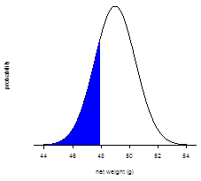
For our 30 samples, the mean net weight is 48.98 g with a standard deviation of 1.433 g. The stated net weight of 1.69 oz is equivalent to 47.9 g. To find the probability that the M&Ms in a randomly selected 1.69-oz bag have a mass less than 47.9 g, we first calculate the deviation, z, taking the mean and the standard deviation for our samples as estimates for μ and σ

\[z=\dfrac{x-μ}{σ}=\dfrac{47.9 -48.98}{1.433} =-0.747\]

and then use the table in Appendix 3 to find the area under the normal curve to the left of 47.9, finding that it is 0.228, or 22.8%; the figure below shows this area highlighted in blue

To decrease this probability to 5%, or 0.050, we use Appendix 3 to find that this corresponds to a z of –1.645. Substituting this into the equation for z gives

\[z= \dfrac{x-μ}{σ}=\dfrac{47.9 -μ}{σ}=-1.645\]

With one equation and two unknowns, there are many possible combinations of mu and sigma that will work. We can place an upper limit on each by maintaining σ as 1.433 and calculating μ

\[\dfrac{47.9 -μ}{1.433} =-1.645\]

and calculating μ as 50.27 g, or by maintaining μ as 48.98

\[\dfrac{47.9 -48.98}{σ}=-1.645\]

and calculating σ as 0.650 g. Given that the average bag has a mean net weight of 48.98 g and a mean number of M&Ms of 56.63, the average plain M&M has a mass of 0.865 g. To increase the mean net weight from 48.98 g to 50.27 g, we need to increase the mean number of M&Ms per bag to 57.92, or we need to decrease the standard deviation by the equivalent of ±0.91 M&Ms.

Investigation 25.

Suppose we arrange to collect samples of plain M&Ms such that each sample contains 330 M&Ms—an amount roughly equivalent to a 10-oz bag of plain M&Ms—drawn from the same population as the data in Table 2. Can we model this data using a normal distribution in place of the binomial distribution or the Poisson distribution? What advantages are there in being able to use the normal distribution? How might you apply this to more practical analytical problems, such as determining the concentration of Pb²⁺ in soil?

When N is equal to 5—as is the case in Investigation 22—it is impossible to use a normal distribution to approximate a binomial distribution because there is no probability, p, where both N × p ≥ 5 and N × (1 - p) ≥ 5 are true. If we increase N to 330, then any value of p that is greater than 0.0152 or that is smaller than 0.984 will allow us to approximate the data using a normal distribution; for the data in Table 2, the smallest value of p is for green M&Ms (0.0647, or 6.47%) and the largest value of p is for brown M&Ms (0.258, or 25.8%); thus, we expect that it is possible to model the data using a normal distribution.

The average count per 1.69-oz bag, λ, of each color of M&M ranges from a minimum of 3.67 for green M&Ms to a maximum of 14.8 for brown M&Ms, neither of which meets the criterion of λ ≥ 5 needed to use a normal distribution to approximate the Poisson distribution. If we increase N from an average of 56.63, for the data in Table 2, to 330, then the average count for any color will increase by 5.83×; thus, the smallest value of λ for any color is 21.3 for green M&Ms, which suggests that it is possible to model the data using a normal distribution.

The primary advantage to us in using the normal distribution is being able to use a single distribution to model diverse types of data, which often simplifies our analysis of data.

A sample of soil consists of many different types of materials—some organic and some inorganic—each of which has a different μ and σ for its concentration of Pb²⁺. Because individual particles of these materials are small, in any reasonable sample the value of N for each particle is sufficiently large that the concentration of Pb²⁺ likely follows a normal distribution even if the underlying distribution of particles follows a binomial or a Poisson distribution.