
9: More on PIB and Orthonormality (Lecture)
- Page ID
- 38876
Last lecture focused on gaining an intuition of wavefunctions with an emphasis on the particle in the box. Specifically, we considered the four principal properties of continuous distributions given in Worksheet 1 and applied it to the particle in the box. This must be mastered for the exam. We want to develop an intuition behind how the energy and wavefunctions change in PIB when mass is increased, when box length is increased and when quantum number n is increased.
We ended the discussion in class focusing on a powerful (blow your mind) fact that the eigenstates of an operator will be orthogonal.
\[\int_{0}^{L}\psi _{m}(x)\psi _{n}(x)dx=0\: \: \: if\: \: \: m \neq n \label{3.5.19}\]
This is really cool as we will see.
Normalization of the Wavefunction
Since wavefunctions can, in general, be complex functions, the physical significance cannot be found from the function itself because \(\sqrt {-1}\) is not a property of the physical world. Rather, the physical significance is found in the product of the wavefunction and its complex conjugate, i.e. the absolute square of the wavefunction, which also is called the square of the modulus.
\[ \psi^*(r , t ) \psi (r , t ) = {|\psi (r , t)|}^2 \label {3.6.1}\]
where \(r\) is a vector (x, y, z) specifying a point in three-dimensional space. The square is used, rather than the modulus itself, just like the intensity of a light wave depends on the square of the electric field.
Probability is a real number between 0 and 1. An outcome of a measurement that has a probability 0 is an impossible outcome, whereas an outcome that has a probability 1 is a certain outcome.
According to Equation \(\ref{3.6.1}\), the probability of a measurement of \(x\) yielding a result between \(-\infty\) and \(+\infty\) is
\[P_{x \in -\infty:\infty}(t) = \int_{-\infty}^{\infty}\vert\psi(x,t)\vert^{ 2} dx. \label{3.6.2}\]
However, a measurement of \(x\) must yield a value between \(-\infty\) and \(+\infty\), since the particle has to be located somewhere. It follows that \(P_{x \in -\infty:\infty}(t) =1\), or
\[\int_{-\infty}^{\infty}\vert\psi(x,t)\vert^{ 2} dx = 1, \label{3.6.3}\]
which is generally known as the normalization condition for the wavefunction.
Normalize the wavefunction of a Gaussian wave packet, centered on \(x=x_o\), and of characteristic width \(\sigma\): i.e.,
\[\psi(x) = \psi_0 {\rm e}^{-(x-x_0)^{ 2}/(4 \sigma^2)}. \label{3.6.4}\]
- Strategy
-
To normalize the wave function \(\psi (x)\) it is important to recognize that
\[\int_{-\infty}^{\infty} \psi_n^* \psi_n dx\]
is the probability of finding a particle in all space, which is 1, or 100%.
- Answer
-
To determine the normalization constant \(\psi_0\), we simply substitute Equation \(\ref{3.6.4}\) into Equation \(\ref{3.6.3}\), to obtain
\[\vert\psi_0\vert^{ 2}\int_{-\infty}^{\infty}{\rm e}^{-(x-x_0)^{ 2}/(2 \sigma^2)} dx = 1. \label{3.6.5}\]
Changing the variable of integration to \(y=(x-x_0)/(\sqrt{2} \sigma)\), we get
\[\vert\psi_0\vert^{ 2}\sqrt{2} \sigma \int_{-\infty}^{\infty}{\rm e}^{-y^2} dy=1. \label{3.6.6}\]
However,
\[\int_{-\infty}^{\infty}{\rm e}^{-y^2} dy = \sqrt{\pi}, \label{3.6.7}\]
which implies that
\[\vert\psi_0\vert^{ 2} = \dfrac{1}{(2\pi \sigma^2)^{1/2}}. \label{3.6.8}\]
Hence, a general normalized Gaussian wavefunction takes the form
\[\psi(x) = \dfrac{e^{\rm{i} \phi}}{(2\pi \sigma^2)^{1/4}}e^{-(x-x_0)^2/(4 \sigma^2)} \label{3.6.9}\]
where \(\phi\) is an arbitrary real phase-angle.
Normalizing the eigenstates of the particle in a box.
- Strategy:
-
To normalize the wave function \(\psi (x)\) it is important to recognize that
\[\int_{-\infty}^{\infty} \psi_n^* \psi_n dx \label{n1}\]
is the probability of finding a particle in all space, which is 1, or 100%.
- Answer
-
The normalization integral (Equation \ref{n1}) can be broken up into three parts, defined by the system's boundary conditions:
\[\int_{-\infty}^{0} \psi_n^* \psi_n dx+ \int_{0}^{a} \psi_n^* \psi_n dx + \int_{a}^{\infty} \psi_n^* \psi_n dx = 1 \]
since \(\psi (x) = 0\) when \(x<0\) and \(x>a\), the first and last integral of the summation of integrals are zero. That leaves
\[N^2\int_{0}^{a} \psi_n^* \psi_n dx\ = 1\]
where \(N\) is the normalization constant. Thus,
\[1=N^2 \int_0^a {\sin}^2(n\pi x/a)dx = N^2(a/2). \label{3}\]
Solving for \(N\) = \(\sqrt{2/a}\). Going back to \(\psi (x) = B\sin(\frac {n\pi x}{a})\), the new equation becomes
\[\psi (x) = \sqrt{\frac{2}{a}}\sin \left(\frac{n\pi x}{a}\right) \label{4}\]
Full Time Dependence
Recall that the time-dependence of the wavefunction with time-independent potential was discussed in Section 3.1 and is expressed as
\[\Psi(x,t)=\psi(x)e^{-iEt / \hbar}\]
so for the particle in a box, these are
\[\Psi _{n}(x)= \underbrace{\sqrt{\dfrac{2}{L}} \sin \dfrac{n\pi x}{L}}_{\text{spatial part}} \overbrace{e^{-iE_nt / \hbar}}^{\text{temporal part}} \label{PIBtime} \]
with \(E_n\) given by
\[E_{n}=\dfrac{\hbar^2\pi^2}{2mL^2}\, n^2=\dfrac{h^2}{8mL^2}n^2 \label{3.5.11}\]
with \(n=1,2,,3...\).
The phase part of Equation \ref{PIBtime} can be expanded into a real part and a complex components. So the total wavefunction for a particle in a box is
\[\Psi(x,t)= \underbrace{\left(\sqrt{\dfrac{2}{L}} \sin \dfrac{n\pi x}{L}\right) \left(\cos \dfrac{E_nt}{\hbar}\right)}_{\text{real part}} - \underbrace{i \left(\, \sqrt{\dfrac{2}{L}} \sin \dfrac{n\pi x}{L} \right) \left(\sin \dfrac{E_nt}{\hbar} \right) }_{\text{imaginary part}}\]
which can be simplified (slightly) to
\[\Psi(x,t)= \underbrace{\left(\sqrt{\dfrac{2}{L}} \sin \dfrac{n\pi x}{L}\right) \left(\cos \dfrac{E_nt}{\hbar}\right)}_{\text{real part}} - \underbrace{i \left(\, \sqrt{\dfrac{2}{L}} \sin \dfrac{n\pi x}{L} \right) \left(\cos \dfrac{E_nt}{\hbar} - \dfrac{\pi}{2} \right) }_{\text{imaginary part}}\]
As discussed previously, the imaginary part of the total wavefunction oscillates out of phase by \(π/2\) with respect to the real part (we call this "out of phase"). This is demonstrated in the time-dependent behavior of the first three eigenfunctions below.
Java simulation of particles in boxes :https://phet.colorado.edu/en/simulation/bound-states
The problem with the standing-wave-on-a-string analogy is that the time dependence of such a standing wave is inherently different from that of a wave function. The time-changing phase of the wave function does not affect its spatial amplitude, as it does with a string. We can thank the fact that the wave function is complex-valued for this. The time evolution for quantum systems has the wave function oscillating between real and imaginary numbers.
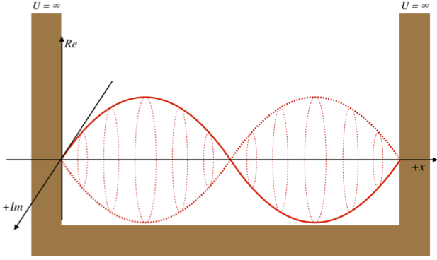
The real and imaginary axes indicated give us a picture of a wave that is circling around the \(x\)-axis, not through it. The displacement of the wave from the axis at a given value of \(x\) doesn't change over time – only its orientation within the complex plane evolves. The shape of the wave function is determined by \(\psi_2\left(x\right)\), and the orientation as it rotates is determined by the time portion, \(e^{-i\omega_2 t}\), with \(\omega_2\) equal to the speed of the "jump rope's" rotation, which is determined by the energy of the state, \(E_2\).
- Think more like this
-

Orthonormality of Wavefunctions
Another important property of the eigenfunctions applies to the integral over a product of two different eigenfunctions. It is easy to see from Figure \(\PageIndex{5}\) that the integral
\[\int_{0}^{a}\psi _{2}(x)\psi _{1}(x)dx=0 \label{3.5.18}\]
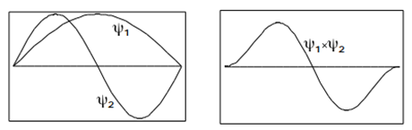
To prove this result in general, use the trigonometric identity
\[\sin\,\alpha \: \sin\, \beta =\dfrac{1}{2}\begin{bmatrix}\cos(\alpha -\beta )-\cos(\alpha +\beta )\end{bmatrix}\]
to show that
\[\int_{0}^{L}\psi _{m}(x)\psi _{n}(x)dx=0\]
if \(m \neq n\).
This property is called orthogonality. We will show in the next Chapter, that this is a general result from quantum-mechanical eigenfunctions. The normalization (Equation \(\ref{3.5.18}\)) together with the orthogonality (Equation \(\ref{3.5.19}\)) can be combined into a single relationship
\[\int_{0}^{L}\psi _{m}(x)\psi _{n}(x)dx=\delta _{mn}\label{3.5.20}\]
In terms of the Kronecker delta
\[\delta _{mn}\equiv \begin{bmatrix}1\; if\; m=n\\ 0\; if\; m\neq n\end{bmatrix}\label{3.5.21}\]
A set of functions \(\begin{Bmatrix}\psi_{n}\end{Bmatrix}\) which obeys Equation \(\ref{3.5.20}\) is called orthonormal.
Back to Expectation Values
The expectation value is the probabilistic expected value of the result (measurement) of an experiment. It is not the most probable value of a measurement; indeed the expectation value may have zero probability of occurring. The expected value (or expectation, mathematical expectation, mean, or first moment) refers to the value of a variable one would "expect" to find if one could repeat the random variable process an infinite number of times and take the average of the values obtained. More formally, the expected value is a weighted average of all possible values.
The quantum mechanical expectation value \(\langle o \rangle\) for an observable, \(o\), associated with an operator, \(\hat{O}\), is given by
\[ \langle o \rangle = \int _{-\infty}^{+\infty} \psi^* \hat{O} \psi \, dx \label{expect}\]
where \(x\) is the range of space that is integrated over (i.e., an integration over all possible probabilities). The expectation value changes as the wavefunction changes and the operator used (i.e, which observable you are averaging over).
In general, changing the wavefunction changes the expectation value of the observable associated with that operator.