18.6: Gibbs Free Energy

Introduction

In the previous section we derived Gibbs Free Energy from the Second Law of Thermodynamics and showed that a system will spontaneously react in the direction that lowers its Free Energy We showed that processes that reduced enthalpy (exothermic processes) or increased the entropy of the system contributed to spontaneity. We also showed that for a system at equilibrium, the change in free energy is zero.

Summary of Free Energy Equations

\[\begin{align} G &=H-TS \\[5pt] \Delta G &= \Delta H -T\Delta S \\[5pt] (\Delta G^o & = \Delta H^o - T\Delta S^o) \\[5pt] \Delta G & = \Delta G^o + RT\ln Q \\[5pt] \Delta G^o & = -RT\ln K \\[5pt] K &=e^{\frac{-\Delta G^o}{RT}} \end{align} \]

Standard State Calculations

Equilibrium Constant at 298 K

Free energy values at standard state can be used to calculate equilibrium constants (using eq. 18.5.6).

Exercise \(\PageIndex{1}\)

Using the table of standard state molar thermodynamic values (Table T.1), calculate the equilibrium constant K for the following reaction at 25^o C.

\[2Ag_2O(s) \leftrightharpoons 4Ag(s) + O_2(g) \nonumber \]

Answer

\[K =e^{\frac{-\Delta G^o}{RT}} \nonumber \]

Noting, \(\Delta G^o_{rxn}= 4(0) + 0 -[2(-11.2kJ/mol)]=22.4kJ \), gives:

\[\large{K=e^{\frac{-22.4kJ/mol}{\left (0.008314 \frac{kJ}{mol \cdot K} \right )298K}} \nonumber =1.19\times 10^{-4}}\]

What does the above problem tell us about the stability of silver in the presence of oxygen? The positive \(\Delta G^o\) tells us that at standard state conditions silver oxidide will not spontaneously form pure silver and oxygen. On the other hand, it says that silver will spontaneously react with oxygen and form the oxidized silver oxide. That is, silver sulfide is stable, and silver is thermodynamically reactive with oxygen. How fast the reaction occurs depends on the kinetics and specifically, the activation energy, but silver will spontaneously form silver oxide.

Equilibrium Constant at other Temperatures

In this class we will consider \(\Delta H_{rxn}\) and \(\Delta S_{rxn}\) to be independent of temperature. This is not a completely legitimate assumption, and is in fact really bad if the system undergoes a phase change.

Exercise \(\PageIndex{2}\)

Consider the reaction

\[N_2(g) +3H_2(g) \leftrightharpoons 2NH_3(g) \nonumber\]

Using Table T1, calculate \(\Delta H^o_{rxn}\) and \(\Delta S^o_{rxn}\) at 25 ºC.

Answer

\[\Delta H^o_{rxn} = 2(-45.9\frac{kJ}{mol}) -[1(0) +3(0)]=-91.8 \frac{kJ}{mol} \nonumber\].

\[\Delta S^o_{rxn} = 2(0.1928 \frac{kJ}{mol \cdot K}) -[1(0.1916\frac{kJ}{mol \cdot K}) +3(0.1307)\frac{kJ}{mol \cdot K}]=-0.1981 \frac{kJ}{mol \cdot K} \nonumber\].

from the previous exercise we get \(\Delta H^o_{rxn}=-91.8 \frac{kJ}{mol}\) and \(\Delta S^o_{rxn}=-198.1 \frac{J}{mol \cdot K}\)

Let's compare these values to the values at 800 K and 1300 K

Temperature (K)	\(\Delta H^o_{rxn}\frac{kJ}{mol}\)	\(\Delta S^o_{rxn}\frac{J}{mol \cdot K}\)
298	-91.8	-198.1
800	-107.4	-225.4
1300	-112.4	-228.0

Exercise \(\PageIndex{3}\)

Calculate \(\Delta G^o_{rxn}\) and K at each temperature using thermodynamic values at that temperature.

Answer

\[\Delta G^o_{rxn}(298K) = -91.8\frac{kJ}{mol} -(298K)(-0.1981)\frac{kJ}{mol \cdot K} = -32.8 \frac{kJ}{mol} \nonumber \\ \large{ K_{eq}= e^{\frac {-\Delta G^o_{rxn}}{RT}} = e^{\frac {-(-32.8 \frac{kJ}{mol})}{(0.008314\frac{kJ}{mol \cdot K} )298K}} =5.62\times 10^5 }\]

\[\Delta G^o_{rxn}(800K) = -107.4\frac{kJ}{mol} -(800K)(-0.2254)\frac{kJ}{mol \cdot K} = 72.92 \frac{kJ}{mol} \nonumber \\ \large{ K_{eq}= e^{\frac {-\Delta G^o_{rxn}}{RT}} = e^{\frac {-(72.92 \frac{kJ}{mol})}{(0.008314\frac{kJ}{mol \cdot K} )800.K}} =2\times 10^{-5} }\]

\[\Delta G^o_{rxn}(1300K) = -112.4\frac{kJ}{mol} -(1300K)(-0.2280)\frac{kJ}{mol \cdot K} = 184.0 \frac{kJ}{mol} \nonumber \\ \large{ K_{eq}= e^{\frac {-\Delta G^o_{rxn}}{RT}} = e^{\frac {-(184.0 \frac{kJ}{mol})}{(0.008314\frac{kJ}{mol \cdot K} )1300.K}} =4.0\times 10^{-8} }\]

So from the above, we see that we have the following K values,

• \(K(298K) = 5.62\times 10^5\)
• \(K(800K) = 2\times 10^{-5}\)
• \(K(1300K) = 4.0\times 10^{-8} .\)

This shows us several things. This is an enthalpy driven reaction and at low temperature it is favorable. But it is entropy impeded, and at high temperature becomes unfavorable.

Often times we do not have thermodynamic values outside of 298 K, and can still approximate \(\Delta G^o_{rxn}\) by using the values of \(\Delta H^o_{rxn}\) and \(\Delta S^o_{rxn}\) at 25 ºC, that is, we assume standard entropy and enthalpy are constant. Lets calculate K_eq at 800 K and 1300 K using the \(\Delta H^o_{rxn}\) and \(\Delta S^o_{rxn}\) at 25 ºC (assuming they are constant over the temperature ranges).

Exercise \(\PageIndex{4}\)

Calculate K_eq at 800 K and 1300 K using the \(\Delta H^o_{rxn}\) and \(\Delta S^o_{rxn}\) at 25 ºC .

Answer

\[\Delta G^o_{rxn}(800K) = -91.8\frac{kJ}{mol} -(800K)(-0.1981)\frac{kJ}{mol \cdot K} = 66.7 \frac{kJ}{mol} \nonumber \\ \large{ K_{eq}= e^{\frac {-\Delta G^o_{rxn}}{RT}} = e^{\frac {-(66.7 \frac{kJ}{mol})}{(0.008314\frac{kJ}{mol \cdot K} )800.K}} =4.4\times 10^{-5} }\]

\[\Delta G^o_{rxn}(1300K) = -91.8\frac{kJ}{mol} -(1300K)(-0.1981)\frac{kJ}{mol \cdot K} = 165.7 \frac{kJ}{mol} \nonumber \\ \large{ K_{eq}= e^{\frac {-\Delta G^o_{rxn}}{RT}} = e^{\frac {-(165.7 \frac{kJ}{mol})}{(0.008314\frac{kJ}{mol \cdot K} )1300.K}} =2.2\times 10^{-7} }\]

Note that now we get

• \(K(800\,K) = 4 \times 10^{-5} \) (it is really \(2 \times 10^{-5}\))
• \(K(1300\,K) = 2.2 \times 10^{-7}\) (it is really \(4 \times 10^{-8}\))

What we see here is that using standard entropy and enthalpy values at 298K gives us reasonably close K values at other temperatures, but the farther away we are from 298, the worse the results. Thus it is common to use the values of \(\Delta H^o_{rxn}\) and \(\Delta S^o_{rxn}\) at 25 degree C for other temperatures to calculate the free energy at the other temperature \[\Delta G^o_{rxn} =\Delta H^o_{rxn} -T \Delta S^o_{rxn} \nonumber \].

Two Meanings of Spontaneous

You will observe that there are two commonly used meanings for spontaneous. In the first context you are asking if a reaction is product favored, in the sense that once equilibrium is achieved, the reactants have converted to products. The second context is that of describing an actual mixture of reactants and products and asking in what direction (if any) will a reaction proceed, that is, is the system Reactant Loaded or Product Loaded.

Product/Reactant Favored Reactions

Here you are looking at the values of \(\Delta G^o_{rxn}\) and K_eq, and asking do the equilibria favor reactants or products

Product Favored Reactions
\(\Delta G^o_{rxn}\)<<0 (it is very negative) and \(K \gg 1\) (it is a very large number).

Reactant Favored Reactions
\(\Delta G^o_{rxn}\) >>0 (it is very large and positive) and \(K \ll 1\) (it is a very small fraction).

Exercise \(\PageIndex{5}\)

Does silver chloride dissolve in water?

Answer

Silver chloride has a very small K, K_sp = 1.8 x 10^-10 .

\[\Delta G^o_{rxn}=-RTlnK=-(0.008314\frac{kJ}{mol \cdot K} )298Kln(1.8\times 10^{-10}) = 55.6kJ/mol\]

Note, from Exercise 5 that for silver chloride, \(\Delta G^o\)=55.6kJ/mol, which is a very large number and corresponds to a very small equilibrium constant, K_sp = 1.8 x 10^-10, and so we would say that silver chloride does not dissolve.

Product/Reactant Loaded Reactions

Here you are given concentrations of reactants and products and need to determine if \(\Delta G\) is greater than, less than, or equal to Zero.

\[\Delta G_{rxn} = \Delta G^o_{rxn} +RT \ln Q\]

Where Q is the reaction quotient. If

\(\Delta G_{rxn} < 0\) - Forward reaction is spontaneous
\(\Delta G_{rxn} >0\) - Reverse reaction is spontaneous
\(\Delta G_{rxn} = 0\) - System is at Equilibrium

This meaning of spontaneous is different than the above meaning, and not stating whether an equilibrium is product or reactant favored, but if a reaction will occur. In the next example we will see that at very dilute (nanomolar) concentrations, even an insoluble salt will dissolve.

Exercise \(\PageIndex{6}\)

Will 100 nmoles of silver chloride dissolve in one liter of water? (Can you make a 100. nM solution of AgCl?)

Answer

As we are given concentrations we need to look at \(\Delta G_{rxn}\) and not \(\Delta G^o_{rxn}\), although we can use \(\Delta G^o_{rxn}\) from the problem above that asked if silver chloride was a soluble salt.

\[\Delta G_{rxn} = \Delta G^o_{rxn} +RTlnQ\]

note, 100nM =100(10^-9M) =1\times 10^-7M, and Q=x².

\[\begin{align}\Delta G_{rxn} &= 55.6kJ/mol -(0.008314\frac{kJ}{mol \cdot K} )298Kln(1.0\times 10^{-7})^2 \nonumber \\ & = 55.6kJ/mol + (-79.9kJ/mol) \nonumber \\ &=-24.3kJ/mol\end{align} \]

What you notice in the above is that there are two terms contributing to \(\Delta G\), that which describes the equilibrium (\(\Delta G^o\)), and that which describes the "loading" of the system, RTlnQ. As silver chloride is a very insoluble salt the first term is 55.6 kJ and positive. If the reaction quotient (Q) is a fraction (meaning few products and many reactants) its log is negative and it contributes towards spontaneity. If it is more negative than the first term is positive, the system is reactant loaded and will spontaneously make products. In the above exercise, the second term was -79.9kJ/mol and so the net \(\Delta G\) is -23.4kJ/mol and the reaction proceeds, with the silver chloride spontaneously dissolving, even though we would call it an insoluble salt.

Driving NonSpontaneous Reactions

In General Chemistry 1, section 5.7.1, Hess's Law we noted that if we coupled two reactions the energy is additive, and this principle also holds for other state functions like Gibbs Free Energy. That is, Free Energies of Reactions are additive. What this means is that a nonspontaneous process (\(\Delta G > O\)) can become spontaneous if it is coupled to a second spontaneous process (\(\Delta G < O\)), if the second process is more negative than the first process is positive.

Consider the decomposition of chalcocite (Copper(i)sulfide).

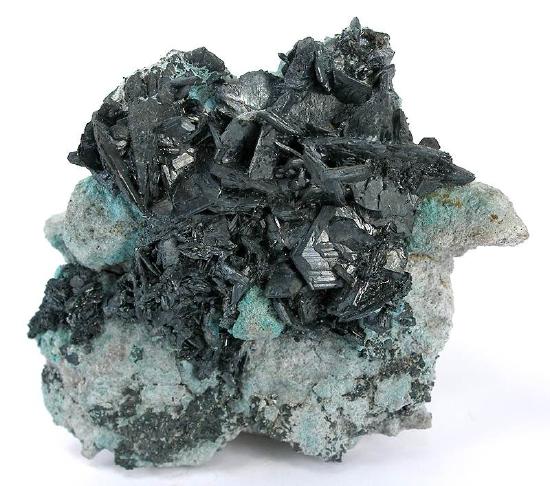
Figure\(\PageIndex{1}\): Chalcocite is a copper ore of Cu₂S, (image from Wikimedia)

Let's say we want to extract the copper from Chalcocite. The first question is, is it stable?

\[ Cu_2S(s) \rightarrow 2Cu(s) + S(s)\]

From the table of standard molar Free Energies of formation (Table T1) the enthalpy of formation of chalcocite is -82.6kJ/mol.

\[2Cu(s) + S(s) \rightarrow 2Cu_2S(s) \; \; \; \Delta G^o_f= -82.6kJ/mol \]

Noting in the above equation that copper and silver are in their standard states (\(\Delta G^o_f = O\)), means the free energy change for the first reaction (18.6.15) is the negative of its \(\Delta G^o_f \), or 86.2kJ. (Note the last value is written in units of kJ and not kJ/mol, as it is related to eq.18.6.15, and the per mole is implicit (per one mole of chalcocite consumed, and per two moles of copper and one mole sulfur produced). This tells us that chalcocite is stable and will not spontaneously form copper and sulfur.

Since we want to extract copper, we could find a reaction that consumes the sulfur, a byproduct, and whose (\Delta G^o_f <-82.6kJ\)) . From (Table T1) we see that \(\Delta G^o_f (\text{sulfur dioxide})\) is -300kJ/mol

\[S(s) +O_2(g) \rightarrow SO_2(g) \; \; \; \Delta G^o_f= -300.1kJ/mol\]

equation 1: Cu₂S(s) --> 2Cu(s) + S(s) ΔH₁ =+82.6kJ (non spontaneous)
equation 2: S(s) + O₂ --> SO₂ ΔH₂ = -300.1kJ (spontaneous)

equation 3: Cu₂S(s) + O₂ --> 2Cu(s) + SO₂ ΔH₃ = 82.6kJ +(-300.1kJ)=-217.5kJ (spontaneous)

Now that we have a thermodynamically feasible process the next step is to find the reaction conditions (temperature, catalysts...) that would allow it to proceed at a viable rate.

Enthalpically vs. Entropically Driving Reactions

Some textbooks and teachers say that the free energy, and thus the spontaneity of a reaction, depends on both the enthalpy and entropy changes of a reaction, and they sometimes even refer to reactions as "energy driven" or "entropy driven" depending on whether ΔH or the TΔS term dominates. This is technically correct but misleading because it disguises the important fact that ΔS_total, which this equation expresses in an indirect way, is the only criterion of spontaneous change.

Consider the following possible states for two different types of molecules with some attractive force:

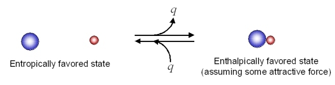
There would appear to be greater entropy on the left (state 1) than on the right (state 2). Thus the entropic change for the reaction as written (i.e. going to the right) would be (-) in magnitude, and the energetic contribution to the free energy change would be (+) (i.e. unfavorable) for the reaction as written.

In going to the right, there is an attractive force and the molecules adjacent to each other have a lower energy state (heat energy, q, is liberated). To go to the left, we have to overcome this attractive force (input heat energy) and the left direction is unfavorable with regard to heat energy q. The change in enthalpy is (-) in going to the right (q released), and this enthalpy change is negative (-) in going to the right (and (+) in going to the left). This reaction as written, is therefore, enthalpically favorable and entropically unfavorable. Hence, it is enthalpically driven.

From Table 18.5.1, it would appear that we might be able to get the reaction to go to the right at low temperatures (lower temperature would minimize the energetic contribution of the entropic change). Looking at the same process from an opposite direction:

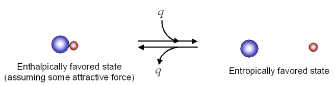
This reaction as written, is entropically favorable, and enthalpically unfavorable. It is entropically driven. From Table 18.5.1 , it would appear that we might be able to get the reaction to go to the right at high temperatures (high temperature would increase the energetic contribution of the entropic change).

Relationship between ΔG and Work

Gibbs Free Energy is the maximum available energy to do non PV work like mechanical or electrical work. Gibbs Free Energy is also very important to understand bioenergetics, and a foundation topic that will be used in upper level chemistry courses. Let's show how \(\Delta G = W_{max}\) for systems at constant pressure and temperature.

\[\Delta G = \Delta H -T\Delta S \; \; \text{at constant temperature} \]
\[\Delta H = \Delta U + P \Delta V \; \; \text{at constant pressure} \]

Substituting the definition of enthalpy (18.6.19) into the definition of Free Energy (18.6.18) gives

\[\Delta G = \Delta U + P \Delta V -T\Delta S \; \; \text{at constant temperature and pressure} \]

From the First Law of Thermodynamics we know

\[\Delta U = Q + W\]
substituting the First Law Internal Energy expression into the free energy equation gives

\[\Delta G = Q + W + P \Delta V -T\Delta S \; \; \text{at constant temperature and pressure} \]

For maximum work, a process must be reversible, and knowing the definition of entropy \(\Delta S = \frac{Q_{rev}}{T}\ \; gives \; Q_{rev}=T\Delta S\), and substitution into the above eq. gives

\[\begin{align}\Delta G & = \cancel{T\Delta S} + W_{rev} + P \Delta V \cancel{-T\Delta S} \; \; \text{at constant temperature and pressure} \\ \Delta G & = W_{rev} + P\Delta V \end{align}\]

The reversible work (W_rev) may be of expansion (W_rev,exp) or non expansion (W_{rev, nonexp}), and noting from section 5.1.4.1, \(W_{rev,exp}=-P\Delta V\) so \(W_{rev}= W_{rev,nonexp}-P\Delta V\). Substituting for reversible work gives:

\[\begin{align}\Delta G & = W_{rev} + P\Delta V \\ &= W_{rev,nonexp}\cancel{-P\Delta V} + \cancel{P\Delta V} \\ & = W_{rev,nonexp} \end{align}\]

This is often written as \[\Delta G = W_{max}, \text{the maximum amount of energy available to do work (at constant T & P)}\]

One of the major challenges facing engineers is to maximize the efficiency of converting stored energy to useful work or converting one form of energy to another. As indicated in Table \(\PageIndex{2}\), the efficiencies of various energy-converting devices vary widely. For example, an internal combustion engine typically uses only 25%–30% of the energy stored in the hydrocarbon fuel to perform work; the rest of the stored energy is released in an unusable form as heat. In contrast, gas–electric hybrid engines, now used in several models of automobiles, deliver approximately 50% greater fuel efficiency. A large electrical generator is highly efficient (approximately 99%) in converting mechanical to electrical energy, but a typical incandescent light bulb is one of the least efficient devices known (only approximately 5% of the electrical energy is converted to light). In contrast, a mammalian liver cell is a relatively efficient machine and can use fuels such as glucose with an efficiency of 30%–50%.

Table \(\PageIndex{2}\): Approximate Thermodynamic Efficiencies of Various Devices

Device	Energy Conversion	Approximate Efficiency (%)
large electrical generator	mechanical → electrical	99
chemical battery	chemical → electrical	90
home furnace	chemical → heat	65
small electric tool	electrical → mechanical	60
space shuttle engine	chemical → mechanical	50
mammalian liver cell	chemical → chemical	30–50
spinach cell	light → chemical	30
internal combustion engine	chemical → mechanical	25–30
fluorescent light	electrical → light	20
solar cell	light → electricity	10
incandescent light bulb	electricity → light	5
yeast cell	chemical → chemical	2–4

Contributors and Attributions

Robert E. Belford (University of Arkansas Little Rock; Department of Chemistry). The breadth, depth and veracity of this work is the responsibility of Robert E. Belford, [e-mail]. You should contact him if you have any concerns. This material has both original contributions, and content built upon prior contributions of the LibreTexts Community and other resources, including but not limited to: