
2.5: Expectation values
- Page ID
- 76707
Expectation Value
We have seen that \(\vert\psi(x,t)\vert^{ 2}\) is the probability density of a measurement of a particle's displacement yielding the value \(x\) at time \(t\). Suppose that we made a large number of independent measurements of the displacement on an equally large number of identical quantum systems. In general, measurements made on different systems will yield different results. However, from the definition of probability, the mean of all these results is simply
\[ \langle x\rangle = \int_{-\infty}^{\infty} x \vert\psi\vert^{ 2} dx \label{ 4.3.5}\]
Here, \(\langle x\rangle\) is called the expectation value of \(x\). Similarly the expectation value of any function of \(x\) is
\[ \langle f(x)\rangle = \int_{-\infty}^{\infty} f(x) \vert\psi\vert^{ 2} dx.\label{ 4.3.6}\]
Postulate 4
The average value of an observable measurement of a state in (normalized) wavefunction \(\psi\) with operator \(\hat{A}\) is given by the expectation value \(\langle a \rangle\):
\[ \langle a \rangle = \int_{-\infty}^{\infty} \psi^* \hat{A} \psi dx = \int_{-\infty}^{\infty} \hat{A} \vert\psi\vert^{ 2} dx \label{4.3.7}\]
If an unormalized wavefunction is used, then Equation \(\ref{4.3.7}\) changes to
\[ \langle a \rangle = \dfrac{ \int_{-\infty}^{\infty} \psi^* \hat{A} \psi dx}{\int_{-\infty}^{\infty} \psi^* \psi dx} \label{4.3.8}\]
The denominator is just the normalization requirement discussed earlier. In general, the results of the various different measurements of \(x\) will be scattered around the expectation value \(\langle x\rangle\). The degree of scatter is parameterized by the quantity
\[\sigma^2_x = \int_{-\infty}^{\infty} \left(x-\langle x\rangle \right)^2 |\psi|^{ 2} dx \equiv \langle x^2\rangle -\langle x\rangle^{2}, \label{4.3.9}\]
which is known as the variance of \(x\). The square-root of this quantity, \(\sigma_x\), is called the standard deviation of \(x\). We generally expect the results of measurements of \(x\) to lie within a few standard deviations of the expectation value (Figure \(\PageIndex{1}\))
.
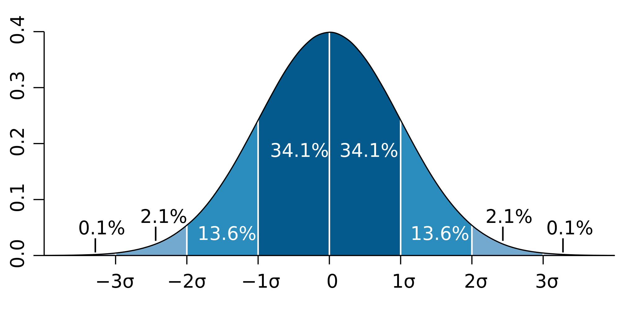
Figure \(\PageIndex{1}\): A plot of a normal distribution (or bell-shaped curve) where each band has a width of 1 standard deviation. image usd with permission from Wikipedia.
Example \(\PageIndex{1}\)
For a particle in a box in its ground state, calculate the expectation value of the
- position,
- the linear momentum,
- the kinetic energy, and
- the total energy
Solution
First the wavefunction needs to be defined. From the particle in the box solutions, the ground state wavefunction (\(n=1\) is
\[\psi = \sqrt{\dfrac{2}{L}} \sin \left ( \dfrac{\pi x}{L} \right )\]
We can confirm that the wavefunction is normalized.
\[\int \psi^* \psi \, d\tau = \int_{0}^{L} \sqrt{\dfrac{2}{L}} \sin \left ( \dfrac{\pi x}{L} \right ) \sqrt{\dfrac{2}{L}} \sin \left ( \dfrac{\pi x}{L} \right ) \, dx = 1\]
Hence, the Equation \(\ref{4.3.7}\) is the relevant equation to use.
The expectation value of the position is:
\[\left \langle x \right \rangle = \int \psi^* x \psi \, d\tau = \int_{0}^{L} \sqrt{\dfrac{2}{L}} x \sin \left ( \dfrac{\pi x}{L} \right ) \sqrt{\dfrac{2}{L}} \sin \left ( \dfrac{\pi x}{L} \right ) \, dx\]
\[=\dfrac{2}{L} \int_{0}^{L} x \sin^2 \left ( \dfrac{\pi x}{L} \right ) \, dx = \dfrac{L}{2}\]
The expectation value of the momentum is:
\[\left \langle p \right \rangle = \int \psi^* \hat{p} \psi \, d\tau =\int_{0}^{L} \sqrt{\dfrac{2}{L}} \sin \left ( \dfrac{\pi x}{L} \right ) \left ( -i\hbar \dfrac{d}{dx} \right ) \sqrt{\dfrac{2}{L}} \sin \left ( \dfrac{\pi x}{L} \right ) \, dx\]
\[= \dfrac{2i\hbar\pi}{L^2} \int_{0}^{L} \sin \left ( \dfrac{\pi x}{L} \right ) \cos \left ( \dfrac{\pi x}{L} \right ) \, dx = 0\]
The expectation value of the kinetic energy is:
\[\left \langle K \right \rangle = \int \psi^* \hat{K} \psi \, d\tau = \dfrac{2}{L} \int_{0}^{L} \sin \left ( \dfrac{\pi x}{L} \right ) \left ( -\dfrac{\hbar^2}{2m} \dfrac{\partial^2}{\partial x^2} \right ) \sin \left ( \dfrac{\pi x}{L} \right ) \, dx \]
\[= \dfrac{\hbar^2 \pi^2}{2mL^2} \dfrac{2}{L} \int_{0}^{L} \sin^2 \left ( \dfrac{\pi x}{L} \right ) \, dx = \dfrac{\hbar^2 \pi^2}{2mL^2}\]
A position "on average" is in the middle of the box (L/2). It has equal probability of traveling towards the left or right, so the average momentum and velocity must be zero. The average kinetic energy must be equal to the total energy of the ground state of the particle in the box, as there is no other energy component (i..e, \(V=0\)).
Expanding the Wavefunction
It is also possible to demonstrate that the eigenstates of an operator attributed to a observable form a complete set (i.e., that any general wavefunction can be written as a linear combination of these eigenstates). However, the proof is quite difficult, and we shall not attempt it here.
In summary, given an operator \(\hat{A}\), any general wavefunction, \(\psi(x)\), can be written
\[\psi = \sum_{i}c_i \psi_i\label{4.3.9A}\]
where the \(c_i\) are complex weights, and the \(\psi(x)\) are the properly normalized (and mutually orthogonal) eigenstates of \(\hat{A}\): i.e.,
\[A \psi_i = a_i \psi_i \label{4.3.10}\]
where \(a_i\) is the eigenvalue corresponding to the eigenstate \(\psi_i\), and
\[\int_{-\infty}^\infty \psi_i^\ast \psi_j dx = \delta_{ij}. \label{4.3.11}\]
Here, \(\delta_{ij}\) is called the Kronecker delta-function, and takes the value unity when its two indices are equal, and zero otherwise. It follows from Equations \(\ref{4.3.8}\) and \(\ref{4.3.11}\) that
\[ c_i = \int_{-\infty}^\infty \psi_i^\ast \psi dx. \label{4.3.12}\]
Thus, the expansion coefficients in Equation \(\ref{4.3.12}\) are easily determined, given the wavefunction \(\psi\) and the eigenstates \(\psi_i\). Moreover, if \(\psi\) is a properly normalized wavefunction then Equations \(\ref{4.3.8}\) and \(\ref{4.3.11}\) yield
\[ \sum_i \vert c_i\vert^2 =1. \label{4.3.13}\]
Collapsing the Wavefunction
Wave function collapse is said to occur when a wave function—initially in a superposition of several eigenstates—appears to reduce to a single eigenstate (by "observation"). A particle (or a system in general) can be found in a given state \(\psi(x,t)\). Suppose now a measurement is performed on the wavefuction to characterize a specific property of the system. Mathematically, an operator \(\hat{A}\) is associated with this measurement process, which you suppose has a complete orthonormal set of eigenvalues:
\[\{ \psi_i \}\]
that is typically an infinite set of functionals that depend on quantum number \(n\). The wavefunction \(\Psi\) can be expand e formula you provided. Now, a set of basis functions can be selected to specifies the wavefunction is the coefficients \(\{c_n\}\) of the expansion. Therefore, if the system is perturbed, then your wavefunction will have another set of coefficients \(\{c'_n\}\).
Contributors
Richard Fitzpatrick (Professor of Physics, The University of Texas at Austin)
- Wikiversity