
4.4: Fluorescence and Phosphorescence
- Page ID
- 398281

\( \newcommand{\vecs}[1]{\overset { \scriptstyle \rightharpoonup} {\mathbf{#1}} } \)
\( \newcommand{\vecd}[1]{\overset{-\!-\!\rightharpoonup}{\vphantom{a}\smash {#1}}} \)
\( \newcommand{\id}{\mathrm{id}}\) \( \newcommand{\Span}{\mathrm{span}}\)
( \newcommand{\kernel}{\mathrm{null}\,}\) \( \newcommand{\range}{\mathrm{range}\,}\)
\( \newcommand{\RealPart}{\mathrm{Re}}\) \( \newcommand{\ImaginaryPart}{\mathrm{Im}}\)
\( \newcommand{\Argument}{\mathrm{Arg}}\) \( \newcommand{\norm}[1]{\| #1 \|}\)
\( \newcommand{\inner}[2]{\langle #1, #2 \rangle}\)
\( \newcommand{\Span}{\mathrm{span}}\)
\( \newcommand{\id}{\mathrm{id}}\)
\( \newcommand{\Span}{\mathrm{span}}\)
\( \newcommand{\kernel}{\mathrm{null}\,}\)
\( \newcommand{\range}{\mathrm{range}\,}\)
\( \newcommand{\RealPart}{\mathrm{Re}}\)
\( \newcommand{\ImaginaryPart}{\mathrm{Im}}\)
\( \newcommand{\Argument}{\mathrm{Arg}}\)
\( \newcommand{\norm}[1]{\| #1 \|}\)
\( \newcommand{\inner}[2]{\langle #1, #2 \rangle}\)
\( \newcommand{\Span}{\mathrm{span}}\) \( \newcommand{\AA}{\unicode[.8,0]{x212B}}\)
\( \newcommand{\vectorA}[1]{\vec{#1}} % arrow\)
\( \newcommand{\vectorAt}[1]{\vec{\text{#1}}} % arrow\)
\( \newcommand{\vectorB}[1]{\overset { \scriptstyle \rightharpoonup} {\mathbf{#1}} } \)
\( \newcommand{\vectorC}[1]{\textbf{#1}} \)
\( \newcommand{\vectorD}[1]{\overrightarrow{#1}} \)
\( \newcommand{\vectorDt}[1]{\overrightarrow{\text{#1}}} \)
\( \newcommand{\vectE}[1]{\overset{-\!-\!\rightharpoonup}{\vphantom{a}\smash{\mathbf {#1}}}} \)
\( \newcommand{\vecs}[1]{\overset { \scriptstyle \rightharpoonup} {\mathbf{#1}} } \)
\( \newcommand{\vecd}[1]{\overset{-\!-\!\rightharpoonup}{\vphantom{a}\smash {#1}}} \)
\(\newcommand{\avec}{\mathbf a}\) \(\newcommand{\bvec}{\mathbf b}\) \(\newcommand{\cvec}{\mathbf c}\) \(\newcommand{\dvec}{\mathbf d}\) \(\newcommand{\dtil}{\widetilde{\mathbf d}}\) \(\newcommand{\evec}{\mathbf e}\) \(\newcommand{\fvec}{\mathbf f}\) \(\newcommand{\nvec}{\mathbf n}\) \(\newcommand{\pvec}{\mathbf p}\) \(\newcommand{\qvec}{\mathbf q}\) \(\newcommand{\svec}{\mathbf s}\) \(\newcommand{\tvec}{\mathbf t}\) \(\newcommand{\uvec}{\mathbf u}\) \(\newcommand{\vvec}{\mathbf v}\) \(\newcommand{\wvec}{\mathbf w}\) \(\newcommand{\xvec}{\mathbf x}\) \(\newcommand{\yvec}{\mathbf y}\) \(\newcommand{\zvec}{\mathbf z}\) \(\newcommand{\rvec}{\mathbf r}\) \(\newcommand{\mvec}{\mathbf m}\) \(\newcommand{\zerovec}{\mathbf 0}\) \(\newcommand{\onevec}{\mathbf 1}\) \(\newcommand{\real}{\mathbb R}\) \(\newcommand{\twovec}[2]{\left[\begin{array}{r}#1 \\ #2 \end{array}\right]}\) \(\newcommand{\ctwovec}[2]{\left[\begin{array}{c}#1 \\ #2 \end{array}\right]}\) \(\newcommand{\threevec}[3]{\left[\begin{array}{r}#1 \\ #2 \\ #3 \end{array}\right]}\) \(\newcommand{\cthreevec}[3]{\left[\begin{array}{c}#1 \\ #2 \\ #3 \end{array}\right]}\) \(\newcommand{\fourvec}[4]{\left[\begin{array}{r}#1 \\ #2 \\ #3 \\ #4 \end{array}\right]}\) \(\newcommand{\cfourvec}[4]{\left[\begin{array}{c}#1 \\ #2 \\ #3 \\ #4 \end{array}\right]}\) \(\newcommand{\fivevec}[5]{\left[\begin{array}{r}#1 \\ #2 \\ #3 \\ #4 \\ #5 \\ \end{array}\right]}\) \(\newcommand{\cfivevec}[5]{\left[\begin{array}{c}#1 \\ #2 \\ #3 \\ #4 \\ #5 \\ \end{array}\right]}\) \(\newcommand{\mattwo}[4]{\left[\begin{array}{rr}#1 \amp #2 \\ #3 \amp #4 \\ \end{array}\right]}\) \(\newcommand{\laspan}[1]{\text{Span}\{#1\}}\) \(\newcommand{\bcal}{\cal B}\) \(\newcommand{\ccal}{\cal C}\) \(\newcommand{\scal}{\cal S}\) \(\newcommand{\wcal}{\cal W}\) \(\newcommand{\ecal}{\cal E}\) \(\newcommand{\coords}[2]{\left\{#1\right\}_{#2}}\) \(\newcommand{\gray}[1]{\color{gray}{#1}}\) \(\newcommand{\lgray}[1]{\color{lightgray}{#1}}\) \(\newcommand{\rank}{\operatorname{rank}}\) \(\newcommand{\row}{\text{Row}}\) \(\newcommand{\col}{\text{Col}}\) \(\renewcommand{\row}{\text{Row}}\) \(\newcommand{\nul}{\text{Nul}}\) \(\newcommand{\var}{\text{Var}}\) \(\newcommand{\corr}{\text{corr}}\) \(\newcommand{\len}[1]{\left|#1\right|}\) \(\newcommand{\bbar}{\overline{\bvec}}\) \(\newcommand{\bhat}{\widehat{\bvec}}\) \(\newcommand{\bperp}{\bvec^\perp}\) \(\newcommand{\xhat}{\widehat{\xvec}}\) \(\newcommand{\vhat}{\widehat{\vvec}}\) \(\newcommand{\uhat}{\widehat{\uvec}}\) \(\newcommand{\what}{\widehat{\wvec}}\) \(\newcommand{\Sighat}{\widehat{\Sigma}}\) \(\newcommand{\lt}{<}\) \(\newcommand{\gt}{>}\) \(\newcommand{\amp}{&}\) \(\definecolor{fillinmathshade}{gray}{0.9}\)This Chapter describes fluorescent spectroscopy based on the QM theory outlined in the previous Chapter. Electron energy levels within the sample define the spectra of absorption as well as of emission (fluorescence and phosphorescence). Relationship between fluorescent spectroscopy and UV range of light is described.
- Understand how irradiation absorption leads to the excitation of electrons in the system
- Distinguish emission via fluorescence from emission via phosphorescence
- Grasp the kinetics effect: why phosphorescence often occurs much slower than fluorescence within the same system
- Become familiar with the processes described by the Jablonski diagram
- Develop a sense of how the average wavelength values for related absorption, fluorescence and phosphorescence are related
Absorption
In a system with quantized energy levels, its particles (e.g. electrons) in general occupy the lowest energy levels/states. An incoming quantum of radiation with the energy E and frequency ν (E = hν) can excite an electron from a lower energy level (ground state) to an unoccupied higher energy level (excited state) if the energy of the incoming quantum (e.g. photon) matches or resonates with the difference between the energy levels of the excited and ground states (E ≥ Eexcited – Eground). Figure IV.4.A shows the processes of irradiation absorption and subsequent emission via two types of pathways, fluorescence and phosphorescence.

If the energy of an incoming quantum is lower than the Eexcited – Eground difference (E < Eexcited – Eground), the absorption of the incoming irradiation will not happen. For example, two incoming quanta of the same energy will not excite a “ground ⇒ excited” transition with the energy double of the individual quantum of radiation.
If the energy of an incoming quantum is equal to the Eexcited – Eground difference (E = Eexcited – Eground), the upward transition will happen and the excited particle (e.g. electron) will have its energy increased. In terms of the quantum description (Schrödinger equation, equation IV.3.1), the potential energy function defining the states of the excited electron will stay the same, but the wave function will change to the one with a higher energy level and different orbital shape.
If the energy of an incoming quantum is greater than the Eexcited – Eground difference (E > Eexcited – Eground), the absorption of the incoming irradiation will take place and the system can go to a higher energy state (excited). If the energy of the incoming quantum is high enough, its absorption might cause major alterations of the system, e.g. bond breakage (excited electrons leave shared molecular orbitals thus depopulating them), or ionization (excited electrons leaving the atom/molecule).
Fluorescence
An electron excited to a higher unoccupied level with energy value E2 can “relax” back to the original ground level E1 (Figure IV.4.A) via a process called fluorescence. Fluorescence takes place rather quickly, in 10-8-10-5 seconds, due to the fact that the excited electron simply comes back to its original ground state without any quantum number alterations apart from the orbital number. During fluorescence, most of the energy of the initial incoming irradiation is emitted back because the excitation and relaxation occur between the same two levels with energies of E2 and E1. Note that the fluorescence emission frequency ν* is somewhat lower than the absorption frequency (ν* < ν) due to inevitable energy losses during absorption and fluorescence.
Phosphorescence
Another pathway through which the energy of excitation can be recovered is called phosphorescence. During phosphorescence, the excited particle (e.g., an electron), first relaxes to another “excited state” with slightly lower energy level of E’2 (E’2<E2). With high likelihood, a spin flip occurs during such a step (E2 ⇒ E’2), which prevents this still excited electron from relaxing back to its original ground state (E1) right away if there is another electron there with the same spin (Figure IV.4.A). Therefore, it will take a substantial time to reverse the spin flip and allow the excited electron to relax back to the ground state. As a result, phosphorescence may last a lot longer than fluorescence: from milliseconds to days and even years, depending on the specific chemical system. Because E’2<E2, the main phosphorescence frequency ν# is smaller than fluorescence frequency ν* (ν# < ν*).
Jablonski Diagram
In real systems, most molecules consist of multiple atoms, which complicates the set of absorption, fluorescence and phosphorescence transitions. In addition, most electronic quantum energy levels (E1, E2, E’2 etc) undergo internal split due to vibrational motion of the relevant nuclei (vibrational relaxation). Thus, the overall picture includes many transitions of each type and many levels and sub-levels. A complete set of relevant transitions for a specific molecule is referred to as the Jablonksi diagram (Figure IV.4.B).
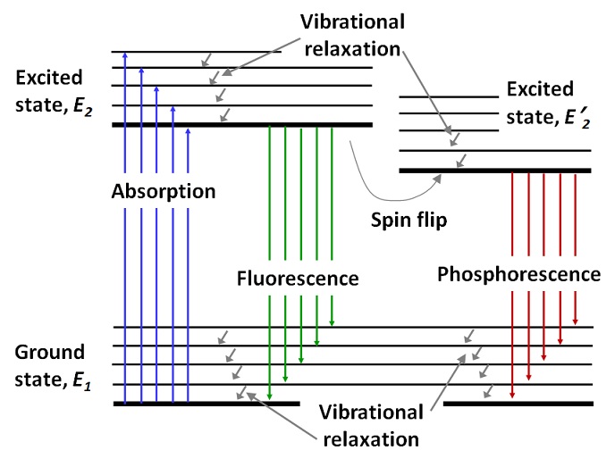
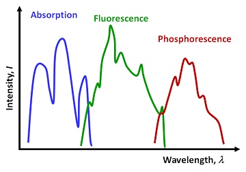
Because of the complexity of the Jablonski diagram for real molecules, the respective absorption, fluorescence and phosphorescence spectra can be messy in terms of the line shapes (Figure IV.4.C). But in general and on average, the relationship between the energy (and thus frequency ν as E=hν) of the absorption, fluorescence and phosphorescence is clear : Eabsorption ≥ Efluorescence ≥ Ephosphorescence. Due to the inverse relationship between the frequency ν and wavelength λ (c=λν), the trends in wavelength values are the opposite: λabsorption ≤ λfluorescence ≤ λphosphorescence (Figure IV.4.C).
Practice problems

In a certain system, three pathways, A, B and C (see figure above), are available for relaxation of excited electrons via fluorescence. The energy change of the downward transitions are as follows:
∆EA= 7.9×10⁻²² kJ, ∆EB= 9.9×10⁻²² kJ, and ∆EC= 4.9×10⁻²² kJ
The number of arrows for each transition is proportional to the probability of each relaxation pathway: the more arrows for the pathway, the more exited electrons follow the pathway to relax.
Practice problem 1. Which pathway(s) generate photons which are capable of disrupting a double –C=C – bond? Justify quantitatively.
Practice problem 2. Provide a spectrum representing the three transitions with the X axis in nm. The spectrum should accurately represent the relative probability of the transitions. Each spectral line should be drawn as a thin vertical bar: assume uniform line widths for all the peaks.
Practice problem 3. Consider the same system at thermal equilibrium. If the system has at its ground state energy levels 1,000,000 moles of electrons, how many electrons will spontaneously occupy all of the “excited” states combined? Justify quantitatively.
Practice problem 4. You are analyzing the Jablonski diagram for two molecules X and Y. Molecule X is double the size of molecule Y (has twice as many atoms). In what ways do you expect the Jablonski diagram for molecule X could be different from that of molecule Y?