
2.1: Heuristic Development
- Page ID
- 203341

1. Traveling waves
Let us account for what we so far understand about the nature of particles.
- With macroscopic measuring devices they appear no different than expected from classical mechanics. That is, for example, their propagation through space (velocity) is related to energy via
\[
E_\text{kinetic} = \frac{1}{2}mv^2
\text{.}\] - A wave-like behavior emerges for low-mass particles at small length scales.
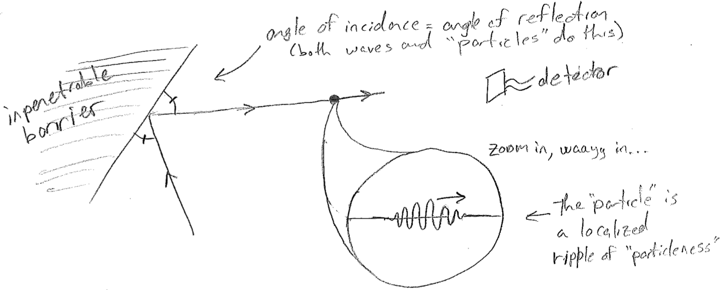
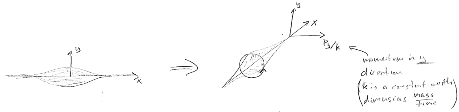
The combination of these facts suggests that perhaps a particle is a wave, but that the wave properties exist at such a short length scale that they are often irrelevant, as illustrated in the figure [#] below. That is, as long as we do not subject the particle to forces with spatial variations similar to the particle wavelength, then any features of the dynamics attributable to a finite wavelength cancel out. Similarly, if a given detector only senses rough position (with an error larger than the spatial extent of the wave), then there is nothing to distinguish a wave from a classical point particle.
The remainder of this subsection explores what kinds of phenomena might be expected from the idea that a particle is actually a microscopic wave, one whose wavelength is inversely proportional to momentum. The approach is heuristic, but not completely deductive. At certain points, the reasoning process will be informed by results of the full quantum theory to come. Nevertheless, some of the most basic qualitative principles will hereby be illustrated with a minimal reliance on equations.
a. wavelength, energy, and tunneling
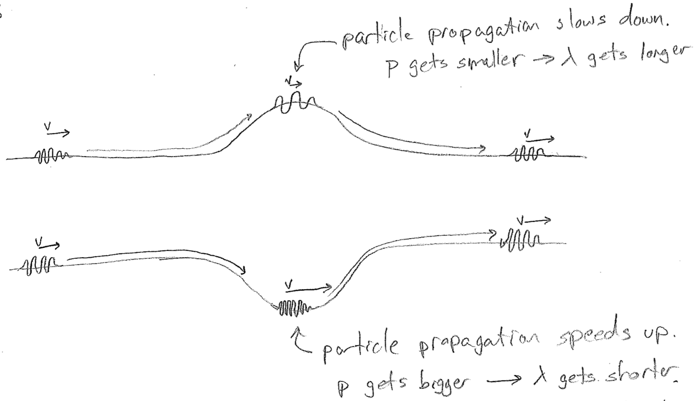
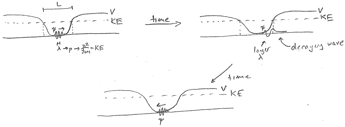
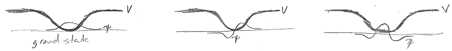
Let us first reflect on what happens to a particle at the microscopic scale as it meets variations in the potential energy, which is illustrated in the figure [#] below. These might be barriers or attractive traps. Most importantly, as the wave slows during traversal of a barrier, we expect the wavelength to increase, and we expect it to decrease as it accelerates into a dip in the potential. In the above figures, the wave has been drawn on top of the barrier or inside the well, in analogy to the familiar hills that humans traverse. However, there is no real meaning to this vertical displacement; assuming the particle is moving in one dimension, it should be confined to a line, simply in a region of high or low potential energy.
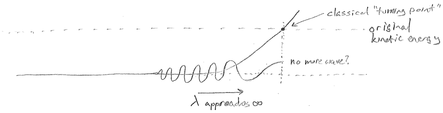
A next reasonable question to ask is: what happens when a wave reaches a point where the potential energy is higher than the kinetic energy that it comes in with? Does the wave simply vanish, as illustrated in the figure [#] below? On the one hand, this makes sense, because the wave should not go to this region classically, but, on the other hand, the abrupt change is questionable. From experiments, we know that particles do have some probability of penetrating barriers that are ostensibly too high. And we also expect that any reasonable wave equation will not allow for such discontinuities. Furthermore, we expect the wavelength to approach infinity first (as the particle slows to a stop), whatever that might mean.
In order to understand how this can work, let us delve further into the notion of a wavelength approaching infinity. The most naive conceptualization would be to have a flat line for the value of the wave. Indeed such a function could be said to have infinite wavelength, such as for \(\cos(2\pi 0 x)=1\) when \(\bar{\nu}=1/\lambda=0\). However, we need not be so restrictive. Consider that one feature of all sinusoidal-like waves (inclusive of ones that vary in wavelength over space) is that they have negative concavity towards the axis along which the propagate. That is, when the wave has a positive value, it is concave-down, but when it has a negative value, it is concave-up. In fact, one of the interesting features of a perfectly sinusoidal wave is that the ratio of the second derivative (the concavity) to the function value is a constant that is directly related to the wavelength \((\bar{\nu}=1/\lambda)\).
\[
\frac{\frac{\text{d}^2}{\text{d}x^2}\sin(2\pi\bar{\nu}x)}{\sin(2\pi\bar{\nu}x)} = -(2\pi\bar{\nu})^2 \label{locallambda}
\]
One could posit, and later we will accept, that this ratio itself provides a reasonable definition of "local" wavelength. In that case, in order to have an infinite wavelength at some point, it suffices that a wave has an inflection point (vanishing second derivative) that is not located at a node (a place where the wave itself crosses zero). This change in concavity results in a function that decays into the barrier, as illustrated in the figure [#] below.
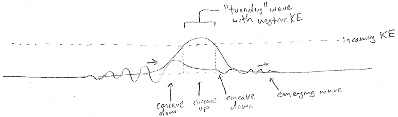
One of the remarkable features of quantum mechanics is that kinetic energy is not strictly positive. According to eq. \ref{locallambda}, in these classically forbidden regions of decaying functions with inverted concavity, the value of \(\bar{\nu}\) must formally be imaginary (which kind of makes sense, since it is not really a "wave" there). If we then insist on using \(E_\text{kinetic}=p^2/(2m)\) with \(p=h\bar{\nu}\), then \(E_\text{kinetic}\) is negative. This allows for a locally energy-conserving mechanism by which barriers higher than the kinetic energy may be “tunneled” through, as opposed to surmounted. This experimentally observed phenomenon is one of the most famous non-intuitive features of quantum physics. Hopefully, it now has a modicum of intuitiveness associated with it in the mind of the reader.
We will later see that the average value of the kinetic energy over an entire wave must be non-negative. This is satisfying to the extent that we expect the totality of a wave to have more classical-like features, so as to facilitate the emergence of classical mechanics from quantum mechanics. The fact that regions of negative kinetic energy are so small and exist so briefly is the reason they are never noticed for macroscopic particles. Consider that the wavelength of \(1.0~\text{kg}\) object moving at \(1.0~\text{m}/\text{s}\) is on the order of \(10^{-34}~\text{m}\). Furthermore, the amplitude of a wave decreases exponentially when penetrating a barrier, crushing the probability of a macroscopic object penetrating a macroscopic barrier.
b. probability and measurement
One of the more subtle consequences of the wave nature of particles is the statistical nature of physical measurements. Much more will be said about measurement during the formal development of quantum mechanics in the next section, but, for now, we will concentrate on measurement of the position of a particle. In particular, we will consider the case of a particle scattering off of a barrier, through which it can be both reflected and transmitted, a phenomenon that will be familiar to many readers in the context of another kind of wave, light, as it meets a half-silvered mirror.
In vague terms the “amount” of wave is conserved, such that if part of a wave traverses a barrier, with the remainder reflected, then the two parts of the wave must sum to the whole. They remain "parts" of one particle. However, detection of the transmitted portion precludes detecting the scattered portion, and vice versa. This means that, under measurement, it behaves as it it were always a single undivided particle, which either reflects or transmits. Nevertheless, quantitative prediction of the probabilities for each demands a wave treatment in the vicinity of the barrier. This so-called wave–particle duality is one of the most frustrating issues in the interpretation of quantum mechanics, whereby waves are necessary, and describe things as being in two places at once, but where such dual realities are never directly observed.
One of the earliest and simplest interpretations of quantum measurement was given by Max Born and Niels Bohr. It simply slates that, under measurement, the square modulus of the wavefunction behaves as if it were a classical probability distribution for the particle.
\[
\rho(\vec{r}) =|\psi(\vec{r})|^2
\]
Most importantly, \(\rho\) is real and non-negative everywhere; if \(\psi\) is real, then \(\rho\) is simply its square. The precise meaning of saying that the “amount” of wave is conserved then amounts mathematically to insisting that
\[
\int_{\text{all}\,\vec{r}} \text{d} \vec{r} ~\rho(\vec{r}) = 1
\]
at all times. Since the reflected part and transmitted part of the wave do not overlap in space when they are far away from the barrier at the detectors, we have, as expected,
\[\begin{align}
1 &= \int_{\text{all}\,\vec{r}} \text{d}\vec{r}~\big|\psi_\text{transmitted}(\vec{r})+\psi_\text{reflected}(\vec{r})\big|^{2} \nonumber\\
&= \int_{\text{all}\,\vec{r}} \text{d}\vec{r}~\Big(\big|\psi_\text{transmitted}(\vec{r})\big|^{2}+\big|\psi_\text{reflected}(\vec{r})\big|^{2}\Big); \quad\quad \psi_\text{transmitted}(\vec{r})\, \psi_\text{reflected}(\vec{r}) = 0 \; \forall~\vec{r}~\text{because non-overlapping}\nonumber\\
&= \int_{\text{all}\,\vec{r}} \text{d}\vec{r}~\rho_\text{transmitted}(\vec{r})+\int_{\text{all}\,\vec{r}} \text{d}\vec{r}~\rho_\text{reflected}(\vec{r}) \nonumber\\
&=P_\text {transmitted}+P_\text{reflected}
\text{,}\end{align}\]
which says that the probabilities of the two allowed, and mutually exclusive, outcomes is one.
The summation or integration to unity of all kinds of measurement probabilities is a general feature of quantum mechanics. The consistency of wave mechanics with the measured probabilities of such outcomes gives credence to the Born interpretation and makes it useful. However, it is important to caution that point-wise particle detectors do not actually exist, and the idea of a particle being at a single point \(\vec{r}\) is also questionable. The particle is best thought of as being a wave. The deeper question is: what does it mean to measure something? The philosophical difficulty here is that it would seem to imply invoking the notion of consciousness (though, strictly, this need not be the case).
c. two-component (complex) waves
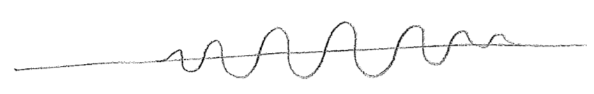
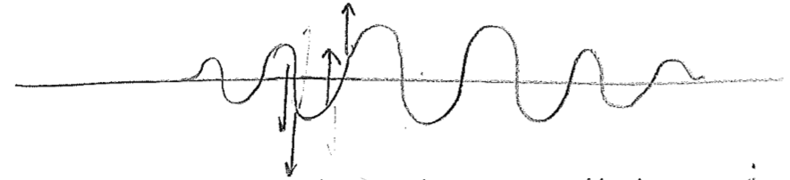
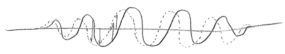
It has been hinted at in the foregoing passage that the wavefunctions for particles may be complex valued. Let us explore the meaning of this. First, consider a snapshot of a wave moving on a string, as in the first figure [#] above. Without an explicit arrows pointing to the right or left, it cannot be determined from the sketch which way the wave is intended to be traveling, but we know that, in reality, the direction of travel must somehow be encoded in the physical state. Similar to particles, this information resides in the momentum of the string. In this case, this is the transverse (up–down) momentum, as illustrated in the second figure [#] above. One can see from this second figure that the wave is moving to the left; as the wave crests move to the left they raise the string to their left, and the troughs similarly lower the string on their left-hand side during leftward travel. These displacements themselves build a wave, shifted by a quarter of a wavelength, as seen in the figure [#] below, where the dotted wave represents the transverse momentum. We can glean from this that the momentum wave being shifted \(\lambda/4\) to the left, relative to the displacement wave, indicates a wave traveling to the left, and being \(\lambda/4\) to the right would mean traveling to the right.
The point that we can abstract from this is that, just as particles have two components to their states (position and momentum), so must waves have two components for their complete description. The situation is not always as simple as having waves for transverse displacement and transverse momentum, as it is for a string. The complete description of electromagnetic waves (light), for example, involves electric and magnetic fields. Only with knowledge of both of these components can the ensuing dynamics be determined. However, for light, directional information follows a more complex rule related to a "right-handed" relationship of the vector-valued electric and magnetic fields to the vector describing propagation. Nevertheless, the point is the same; two wave components are necessary to have a complete dynamical description of a wave (in any number of dimensions), and we can infer from this that our discussion of particle waves has been incomplete, and, to wit, we have so far needed to rely on right–left directional arrows to indicate the intended direction of travel.
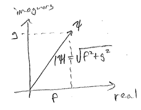
Unlike the case of both waves on strings and electromagnetic waves, the two components of a matter wave for a particle do not have separate physical interpretation. They are simply two components of a single wave, whose spatial relationship to one another plays the role of direction keeper. For such a purpose complex numbers are convenient. A complex number may be thought of as simply a two-component number
\[
(a,b) \quad \rightarrow \quad z=a+\text{i} b
\]
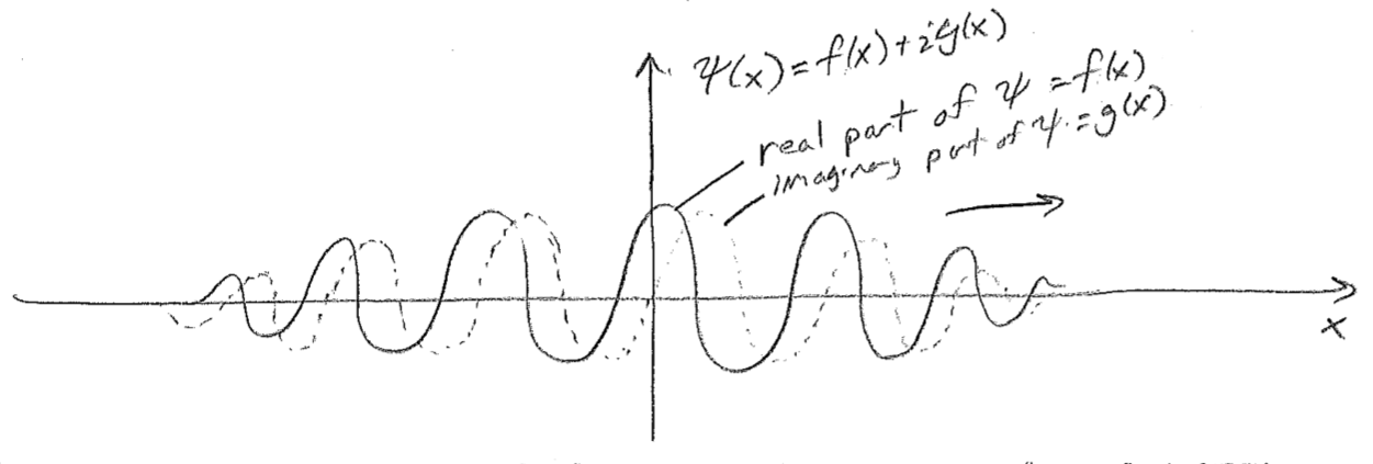
Treating these two components as one complex number is just convenient under certain circumstances (explored in more detail later). Using such a construction, a typical plot for a right-moving wave, \(\psi(x)=f(x)+\text{i}g(x)\), appears in the figure [#] above, where the imaginary component "leads" the real component in the direction of travel. At every point \(x\), \(\psi\) may be thought of as a two-component vector \((f,g)\), and these components feature in the probability density as
\[\begin{align}
\rho(x)
&=|\psi(x)|^2 \nonumber\\
&=\psi^{*\!}(x) ~ \psi(x) \nonumber\\
&=\big(f(x)-\text{i} g(x)\big)\big(f(x)+\text{i} g(x)\big) \nonumber\\
&=(f(x))^{2}+\text{i} f(x) g(x)-\text{i} f(x)g(x)+(g(x))^{2} \nonumber\\
&=(f(x))^{2}+(g(x))^{2}
\text{,}\end{align}\]
where \(\psi^{*\!}(x)\) denotes complex conjugation (changing the sign of the imaginary part). Taking \(|z|^2 = z^*\,z\) is known as taking the square modulus, literally the square of the modulus \(|z|\) of the 2-vector represented by \(z\). Modulus is just another word for length or norm, and so \(|\psi(x)|\) has interpretation as the norm, or overall size, of the 2-vector value of the wavefunction \(\big(f(x),g(x)\big)\) at any point, as illustrated in the figure [#] below.*
* Footnote
In order to emphasize the lack of physically distinct meaning of the real and imaginary components of a wave, consider multiplication of a right-moving plane wave (in 1D) by a constant with square modulus of one.
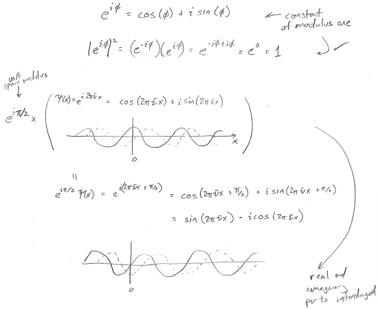
Now consider that, regardless of the form of \(\psi(x)\), such a multiplication can never change the probability density.
\[
\rho(x) = \left(e^{-\text{i} \pi / 2} \psi^{*}(x)\right)\left(e^{\text{i} \pi / 2}\psi(x)\right)=\psi^*(x)\psi(x)=|\psi(x)|^{2}
\]
We will later show that no properties are changed by such a multiplication of the wavefunction. Therefore, there is ambiguity to what the real and imaginary parts are. In other words, one should not try to think of one as more important or real than the other other. Complex numbers are just a book-keeping tool, and the notions of "imaginary" and "real" are just formalities.
d. position and momentum uncertainty
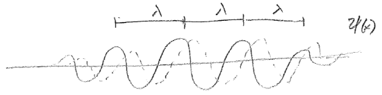
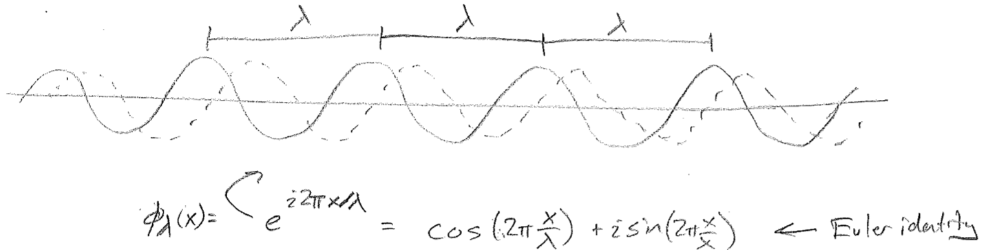
The final major aspect of traveling waves that we will explore qualitatively is known as the Heisenberg uncertainty principle. Let us consider the momentum of a localized wave with fixed \(\lambda\), as shown in the first of the figures [#] above. Clearly, this is not identical to a infinite plane wave with that same \(\lambda\), illustrated in the second figure [#] above. The latter unambiguously has definite wavelength and therefore represents a wave of precise momentum. The former localized wave \(\psi(x)\) can only be produced as a sum of all such plane waves, via
\[
\psi(x) = \sum_{\text{all}\,\lambda} c_{\lambda}\, \phi_{\lambda}(x)
\text{.}\]
where \(\phi_\lambda(x)\) is a plane wave of wavelength \(\lambda\). In reality, "\(\text{all}~\lambda\)" is over a continuous variable and this should be written as an integral, and the best choice for the integration variable is not \(\lambda\) but \(1/\lambda\) (\(\bar{\nu}\)). We will not take up these details now, but this is called Fourier transformation. (It should be noted that, similar to having a particle at a single point, the definite-momentum plane waves themselves are not physically realizable particle states, since their infinite probability distributions cannot be integrated.)
The conclusion is that confining \(\psi(x)\) to a finite spatial interval has come at the cost of summing up waves of different momenta, thereby introducing an uncertainty in the momentum. It needs to be clear that this is a fundamental uncertainty. It is not the result of lack of knowledge of something that has a definite value, but rather, it is a reflection of the fact that the particle does not have a precise momentum, just like it does not have a precise location. The wave contains a distribution or spread of both locations and momenta. The mathematics of Fourier transforms illustrates the trade-off as
\[
\sigma_{x} \sigma_{\bar{\nu}} \geq \frac{1}{4 \pi}
\text{,}\]
which is written in terms of the momentum (\(p=h\bar{\nu}\)) as
\[
\sigma_{x} \sigma_{p} \geq \frac{\hbar}{2}
\text{.}\]
where, again, \(\hbar = h/(2\pi)\). Here, \(\sigma\) indicates the root-mean-square-deviation (RMSD) of the implied spatial and momentum probability distributions. This relationship, in particular the second form of it, is known as the Heisenberg uncertainty principle. It says that, as position is known more precisely, the momentum must be fundamentally less certain, and vice versa. A wavefunction for which the equality holds (as opposed to the inequality) is said to be transform limited, with reference to the underlying Fourier transform.
2. Standing waves
a. the ground state
In order to understand the nature of trapped particles as standing waves, let us perform a “Gedanken experiment” (German for “thought experiment”), where we use our understanding so far to think about our expectation under a new circumstance.
Let us start with a wavepacket at the “bottom” (center) of an attractive potential energy well, but not allow it sufficient kinetic energy to escape the well. Since the “barrier” to escape is infinitely wide, no part of the wave will ever be found traveling outside the well (past the turning points, in the classically forbidden region). This is illustrated as a time series in the figure [#] below. For simplicity, only the real component of the wave is drawn in this figure. Most importantly, as the wave approaches the end of its allowed travel and reverses direction, its wavelength increases when it penetrates the high-potential region, and the decaying part of the wave is a visible fraction of its total positional spread at that time.
Now, let us take the limit of this model as we lower the kinetic energy, so that the initial wavelength becomes longer and eventually reaches the length scale of the trap itself. We begin by letting \(\lambda \approx L\), where \(L\) is the approximate dimension of the trap as shown in the figure [#] below. This time, both the real and imaginary parts of the wave are drawn because it begins to be important. At such low energies, the wave is spread over the whole trap at all times. The decaying parts of the wave on either end are now on the same length scale as the large-amplitude bulge in the middle. Given a node in the middle of the real part, the imaginary part must be maximal there (the maxima of the two components are offset by \(\sim\lambda/4\) for a traveling wave). Now, there is not enough room to fit a full oscillation of the imaginary component before it enters the flanking decaying regions.
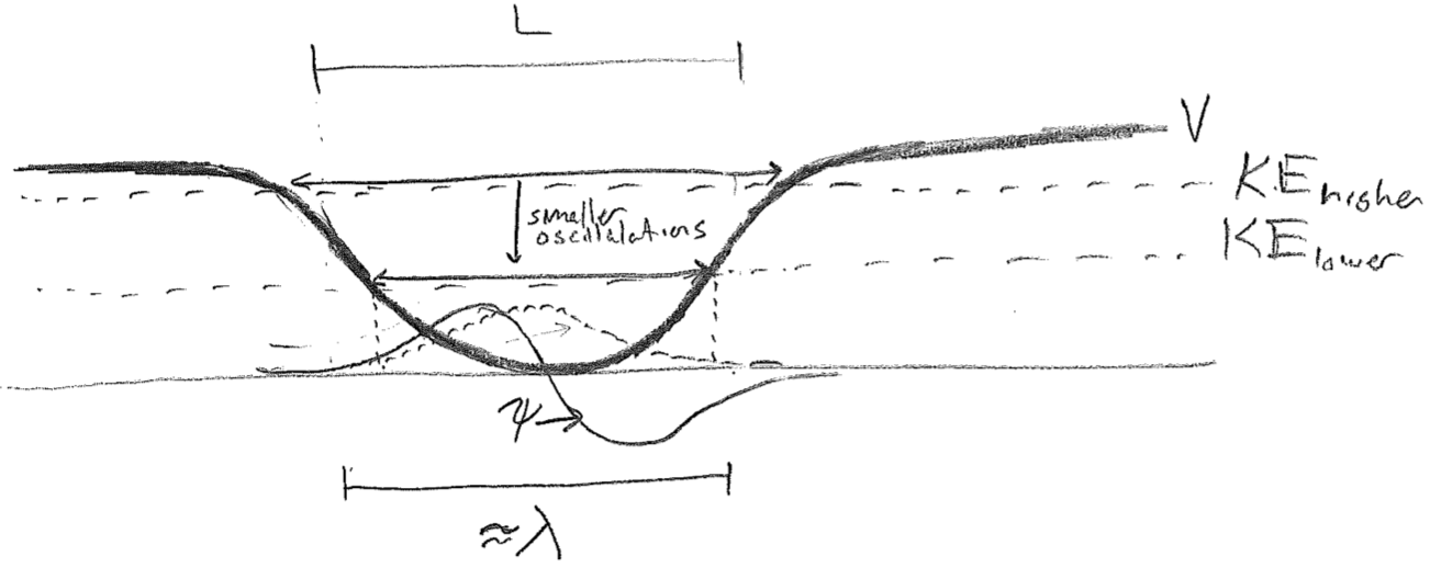
An additional consequence of the positional indeterminacy of the particle wave is that the magnitude of right-left oscillations of the central probability maximum will be smaller than the estimate obtained by locating the classical turning points at this same energy. We appear to be heading towards some kind of limit that has no classical analogy. The wavelength cannot tend toward infinity, or else it will penetrate too far into the potential to be consistent with having low energy. At the same, as we reach the limit of the longest wavelength that the box can support, motion will apparently have ceased. The wave can go no lower in energy, and it just sits in this state motionless, indefinitely. This is known as the ground state.
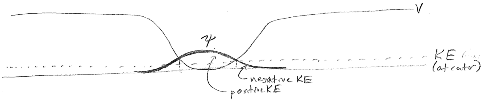
Though we have indicated that waves may be complex (contain \(\text{i}\) where \(\text{i}^2 = -1\)), we never insisted that they must always be so. Indeed, the horizontal offset of real and imaginary components serve to indicate direction of travel, which we have just come to the conclusion ceases at low enough energy. The lowest-energy wave supported by the trap is, in fact, representable as entirely real (or entirely imaginary, etc., since global phase has no consequence), having roughly one half wavelength inside the well, as illustrated in the figure [#] below.
The very existence of a ground state can be thought of as a careful balance between kinetic and potential energies. To decrease the potential energy, the wave would have to contract toward the center. This would give it a shorter effective wavelength and raise the kinetic energy faster than the potential energy decreases. This increase of kinetic energy upon localization is also reflected in the Heisenberg uncertainty principle \(\sigma_{p} \geq \hbar/(2 \sigma_x)\) because shrinking \(\sigma_x\) increases the momentum uncertainty (and therefore kinetic energy). Importantly, this ground state has nonzero kinetic and potential energies. The energy of the ground state of a particle is sometimes called zero-point energy. "Zero" here refers to the fact that this residual energy is present even at zero absolute temperature. The positional spread of the ground-state wavefunction is sometimes said to be due to zero-point motion, rather erroneously.
A striking feature of quantum mechanics has hereby presented itself. In addition to the fact that (local) kinetic energy is not strictly positive, the presence non-zero average kinetic energy does not mean that a particle is moving through space! That said, it is appropriate to note that, although the momentum is not zero (because of finite "wavelength") there is no net direction to the wave; indeed, it is right–left symmetric. In the sense the wave can be said to have momenta (plural because of Heisenberg uncertainty), the average must be zero because it is not traveling.
Before proceeding with more of the development of the concepts of standing particle waves, let us pause to marvel at how, already, with very few equations, we can understand the resolution to one of the outstanding mysteries of the early 20th century. Quantum mechanics, which was formulated to explain various results suggesting that particles act as waves, can be used to directly address the conundrum of electromagnetically unstable planetary-like atoms, arrived at as a result of Rutherford's experiments. In fact, the electron does reside centered on top of the nucleus, but it does not do so as a point particle and, therefore, it does not release an infinite amount of energy in doing so. It would actually cost an infinite amount of energy to compress the electronic wavefunction to a single point. In spite of the strong Coulombic draw, electrons are distributed over finite volumes, thereby giving atoms finite volumes. Only an infinitesimal part of the wave is at the singularity (infinity) in the potential, where the local kinetic energy exhibits a cancelling divergence (discussed later), leaving the energy finite.
b. wave oscillations
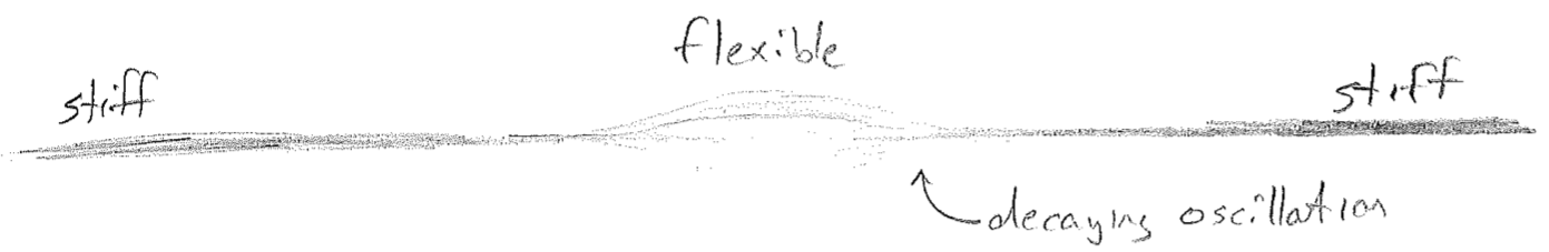
We have now arrived at an interpretation of trapped particles as standing waves, waves whose shapes do not change with time; they have arisen by taking limits of traveling particle waves. To complete the analogy of particle waves to familiar waves on a string, we might ask what it is that can smoothly disallow a wave on a string from escaping a certain region, thus playing the role of potential energy? It is worthwhile to complete this analogy, since we will later reverse it to again enlighten us about particles. The answer is that the string becomes slowly stiffer away from the region of oscillation, as illustrated in the figure [#] below.
The similarities of a trapped particle wave to a wave on an inhomogeneous string are immediately noticeable in terms of their shapes, but an obvious question presents itself. Does a particle wave also oscillate, say "up and down,” whatever that might mean? The answer to the question just posed is yes, no, and sort of, which we will take in turn. It depends on what one means by "up" and "down." For a string, the displacement occurs in the same 3D space in which the string itself lives, and, for light, the oscillating electromagnetic field vectors also have spatial direction, but, for a particle, there is simply some auxiliary particle field that can have a small or large (and negative or positive) value at every point in space. In a sense, yes, this field oscillates up and down, but it there is no spatial direction associated with it.
Now we come to the "sort of" part. It is important here to remember that particle waves are two-component (complex-valued) waves, so that the deviations of the particle field from zero, which constitute the wave, are more complicated than simply "up" (positive) or "down" (negative). But recall that we have argued earlier that all waves have multiple components, including waves on strings. In that earlier context, we addressed how these components keep track of direction of travel, but now we will see something even more important.
Consider again a wave on a string. As the sting temporarily passes through being flat, has the wave disappeared? The answer is, in an obvious sense, yes, but in a less obvious sense, no, when the transverse momentum of the string is considered. The displacement and momentum waves have the same shape, or waveform (because the maximum momentum at any position on the string scales with the maximum displacement there). Furthermore, when the displacement wave is minimized, the momentum wave is maximized. So, in a sense, the wave on a string is simply transitioning between being a displacement wave and a momentum wave. With the correct unit conversions, it can be envisioned as "rotating" between these two axes, as seen in the figure [#] above. When both are taken together, the wave never disappears. As respects a matter wave, such a wave can in no sense disappear or the particle would vanish. It avoids doing so by alternating between being purely real and purely imaginary, rotating constantly in the complex plane as shown in the figure [#] below.
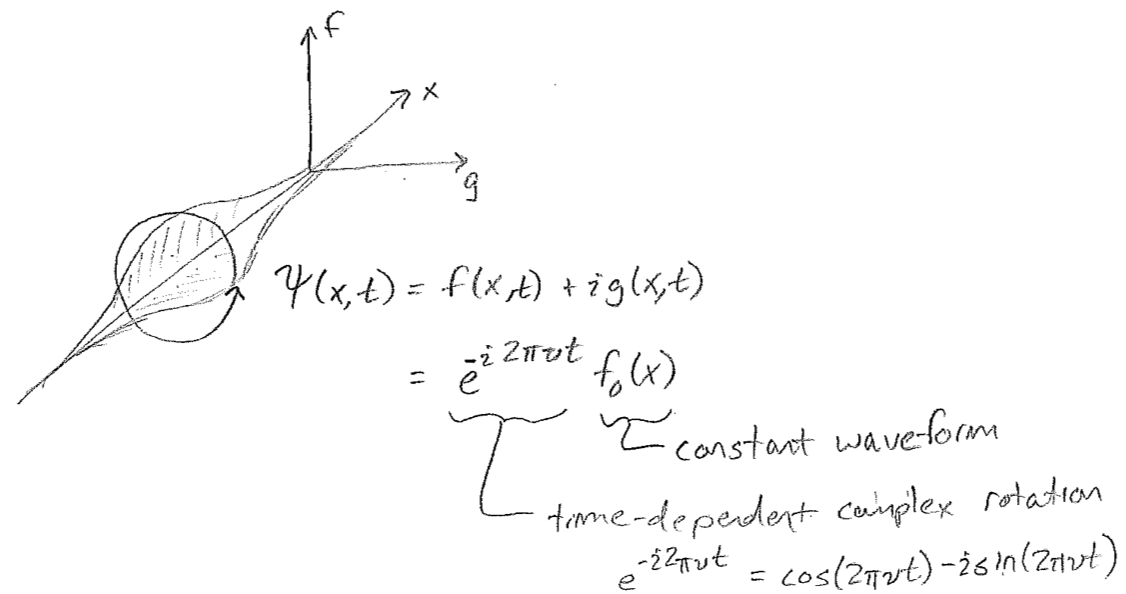
In the course of rotating between real and imaginary, an initially real and positive wave will eventually be the negative of itself and then return to real and positive. So it oscillates between positive and negative (as one expects for a wave on a string), at some frequency \(\nu\), but without ever passing through zero. It goes around zero in the complex plane, preserving the size and shape of the waveform at all times. A useful concept is to interpret \(\text{e}^{\text{i}\phi}\) as a generalization of sign \((\pm)\), which can always be replaced with multiplication by \(\pm 1\). This generalization is called phase. As with \(\pm 1\), \(\text{e}^{\text{i}\phi}\) has size (modulus) of one; however, there are an infinite number of choices for the phase, corresponding to angle in the complex plane. In fact, two such choices are \(\text{e}^{\text{i}0}=+1\) and \(\text{e}^{\text{i}\pi}=-1\). Multiplication of a number or function by a constantly changing phase factor will cause it to rotate/oscillate in the complex sense.
c. boundary conditions and quantization
Now that we have firmly established the idea of a trapped quantum particle as corresponding to a standing wave on the matter field, let us now change the parameters of the problem to an example that is less qualitatively friendly, but easier to work with analytically. The name of this famous model is “particle in a box.” We will introduce it by its analogue on a string. Consider a string, which, rather than getting stiff gradually, becomes stiff suddenly at two end points. For that matter we should just mount a homogeneous string between two fixed points, as done in the idealization of many a musical instrument, for example, a guitar. The fundamental oscillation and the first few overtones are shown in the figure [#] below, along with an arbitrary chaotic wave that could hypothetically be produced.
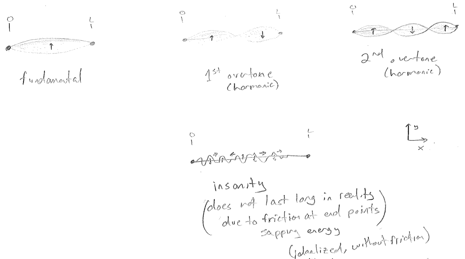
In the last case of an arbitrary wave, it becomes relevant to think of what the equation of motion looks like (idealized, without friction). That is, for a given wave, describable by \(y(x)\) and \(p_\text{y}(x)\) (where the transverse displacement and momentum are taken to be in the \(\text{y}\) direction), what controls the dynamics, that is what controls \(\partial y(x) /\partial t\) and \(\partial p_\text{y}(x)/\partial t\)? Without going into details, the answer is that \(\partial y/\partial t\) depends linearly on \(p_\text{y}\), and \(\partial p_\text{y}(x)/\partial t\) depends linearly on \(y\). This is notably similar to the structure of Hamilton’s equations for a particle. The consequence of this linearity is that adding together any two solutions to the wave equation yields another solution to the wave equation because the wave appears to the first power on both sides of the equation of motion. The argument also works in reverse; any solution to the wave equation, such as the hectic one drawn, may be decomposed as a sum of other solutions to the wave equation. In particular, it is convenient to choose the standing waves, which have well-defined frequencies and constant waveforms, giving, for such a wave
\[
y(x, t)=\sum_{n=1}^{\infty} c_{n} \cos (2 \pi \nu_n t)\,\sin \left(n \pi x/L\right)
\text{.}\]
At \(t=0\), each of the \(\cos (2 \pi \nu_n t)\) terms is equal to \(1\), and adding up the standing-wave spatial functions \(\sin(n \pi x/L)\) with the coefficients \(c_{n}\) produces the initial wave. However, each of the standing waves oscillates with its own frequency \(\nu_n\), changing the shape of the wave over time and yielding its dynamics.
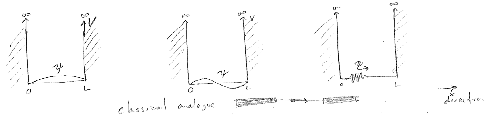
The guitar-string problem maps directly on to a quantum particle trapped in a 1D “box.” A box in 3D is a volume, from which a particle cannot escape. In 1D, it is a line segment from which it cannot escape. This is enforced by potential energy barriers on each end that shoot suddenly to infinity. Since infinitely negative kinetic energy would be required for any penetration into the walls, the rate of decay of the wavefunction is infinitely fast, and we have a pair of boundary conditions, insisting that the wave goes to zero at the ends of the box, as with the guitar string. Also similar to a string, many modes of oscillation that obey these conditions are supported inside the box, as illustrated in the figure [#] below.
We will later see that the wave equation for a matter wave (the Schrödinger equation) is also linear in the wavefunction \(\psi\). This means that any bound or trapped particle can be expressed as a superposition (a sum) of standing matter waves, called stationary states (due to the time independence of any associated properties). As with the modes of a guitar string, the standing waves for a particle in a 1D box have the spatial form
\[
\psi(x) ~\propto~ \sin \left(n \pi \frac{x}{L}\right)
\]
The wavelength for these is well defined as
\[
\lambda_{n}=\frac{2 L}{n}
\text{,}\]
giving a well-defined (absolute value of the) momentum
\[
|p_{n}|=\frac{h}{\lambda_{n}}=\frac{n h}{2 L}
\]
and energy (assuming the potential is zero where it is not infinite)
\[
E_{n}=\frac{p_{n}^{2}}{2 m}=\frac{n^{2} h^{2}}{8 m L^{2}}
\text{.}\]
The wave associated with \(n=1\) is the ground state, and the other states are called excited states, due to their higher energies. We now have come almost full circle back to the origins of quantum mechanics. Recall that the wave nature of matter was invoked as a way to account for quantization of energy, both to attempt to put material on the same footing as light waves (which comes in quanta of \(h\nu\)) and to explain the existence of the mysteriously stable Bohr orbits.
The discussion above demonstrates a central feature of the wave nature of matter. Boundary conditions result in discrete stationary solutions (standing waves) to a wave equation, and this results in the quantization of every measurable property of bound/trapped particles, including energy. This is the origin of "quantum" in the terms quantum theory and quantum mechanics. The relaxing of boundary conditions can also explain why quantization is not observed at the macroscopic scale. As one piece of the transition to classical mechanics, consider that the energies for the particle in the box form a continuum (any value is allowed) as \(L\rightarrow\infty\) or \(m\rightarrow\infty\). Quantum theory is relevant to small things.
It is worth pausing to note that boundary conditions can take many forms. In the case of the smooth finite well, a bound wave must decay into the barrier and approach zero. This is an asymptotic boundary condition, which also leads to quantization, as illustrated by the discrete bound states in the figure [#] below. The energies are harder to predict for such a model, but there are certain regularities, like an increasing number of nodes with increasing energy. We can also make a connection to the atomic model of Bohr and De Broglie, in which periodic boundary conditions were proposed to explain why only certain orbits were stable, ones where the wave repeated itself upon each circuit. Although this model of the atom was theoretically incomplete, we will meet such periodic boundary conditions again.
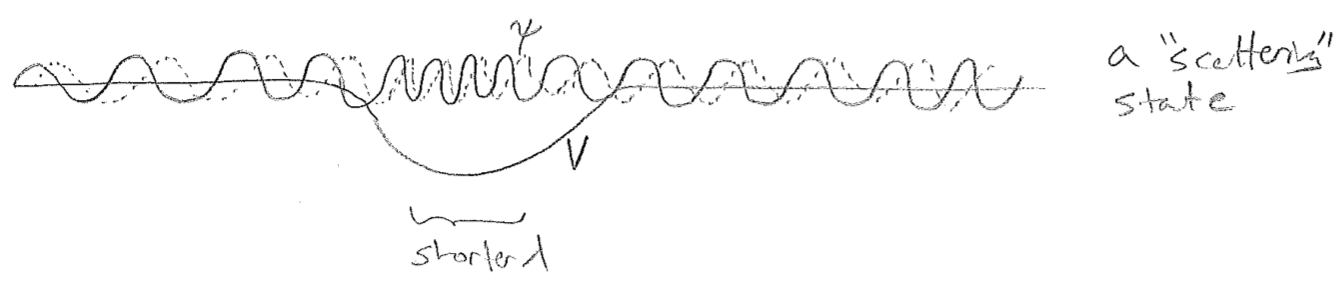
As a final comment about the wavefunctions, it is important to realize that the number of bound states supported depends on the potential. Some finite-depth potentials support only a finite number of bound states. Other finite-depth potentials can support an infinite number of states, which are still discrete, in spite of being ever more closely spaced. In either case, above the escape energy, a true continuum of traveling waves emerges. One can also find stationary states above the escape energy, however, and these are useful as a basis to describe traveling waves as superpositions. These states, called scattering states, cannot be mapped onto a countable set, and they also cannot be normalized (scaled so that their probability density integrates to one). They asymptote to plane waves in 1D, as illustrated in the figure [#] below.
3. Dynamics, energy and spectroscopy
We have just seen how the dynamics of trapped particles may be decomposed into the standing waves supported by the trap, each with its own frequency. Let us now be clear about the relationship between frequency and energy. It is not an accident that the standing waves (having well-defined frequency) for a particle in a box also have well-defined energy. In quantum mechanics, frequency and energy are fundamentally the same. Let us illustrate this in the context of spectroscopy, which uses the light–matter interaction to probe the energy levels of matter.
If standing matter waves with two different frequencies \(\nu_1\) and \(\nu_2\) are interfering, then the resulting time-dependent probability density will have oscillations at a frequency equal to \(\nu_2-\nu_1\) (assume \(\nu_1<\nu_2\)). The details of this will be explored more later; consider now just that if \(\nu_1=\nu_2\), there would be no change in the interference pattern, since the waves oscillate together. So all measurable properties associated with the presently discussed state of the particle will oscillate at the frequency \(\nu_2-\nu_1\). This could potentially include a dipole moment, which would be responsible for the emission of light, clearly with frequency \(\nu_2-\nu_1\). This light would then be associated with a photon energy of \(h(\nu_2-\nu_1)\). Putting this all together, starting with conservation of energy (which we assume), we obtain
\[\begin{align}
\Delta E_\text{matter} &= -h\nu_\text{light} \quad\quad \text{(for emission)}\nonumber\\
E_{1}-E_{2} &= -h(\nu_{2}-\nu_{1}) \nonumber\\
\therefore \quad E_1 &= h\nu_{1} \nonumber\\
E_2 &= h\nu_{2}
\text{,} \end{align}\]
which makes sense if \(E_2>E_1\) (where \(E_n\) is the energy of the standing wave associated with frequency \(\nu_n\)). For absorption, the negative sign may be removed in the second line, and the energy levels swapped, giving the same final result. What this shows is that \(h\) is a universal constant relating energy to frequency, also for oscillations of matter. This condition of matching the frequencies of light to oscillation frequencies in matter is called the Bohr resonance condition.
Finally, we note that, in the forgoing analysis, only relative energies and frequency differences have appeared. Indeed, absolute energies and frequencies for individual states are not meaningful. Recall that, in classical mechanics, one may add an arbitrary constant to the potential energy function, and this does not violate the principle of energy conservation, nor does it change any of the forces (derivatives of the potential) that dictate the dynamics. Although it is difficult (impossible?) to formulate quantum mechanics in terms of forces without recourse to a potential, the arbitrariness of this potential is a feature, which is then inherited by classical mechanics. However, only energy differences have any effect on observables. Consider, as an example \(\rho(x)=|\psi(x)|^{2}\). The probability density \(\rho\) is independent of the change of sign/phase of \(\psi\), so one can add an arbitrary constant to its energy, and therefore its oscillation frequency, without changing anything measurable.