
1.2: The State of Physics around Year 1900
- Page ID
- 202855

1. Particles
a. Newton's and Hamilton's equations of motion
In 1687 Isaac Newton had published Principia Mathematica, which is the foundation of the classical mechanics of particles (classical mechanics excludes relativistic and quantum effects). In this work are found his laws of motion, and the famous equation
\[
\vec{F}(t)=m \, \vec{a}(t) \label{Newton}
\text{,}\]
which says that the acceleration \(\vec{a}\) of a body is proportional to the force \(\vec{F}\) acting on that body at time \(t\), and the proportionality constant is the inverse of the mass \(m\) (when moved to the other side of the equation). This accounts for the resistance of heavier bodies to a change in motion, called inertia. Newton's laws of motion were abstractions gleaned from observing planets. In addition to helping lay the foundations of calculus, Newton also formulated the universal law of gravitation to describe planetary motions. The law of gravitation says that the attraction between two bodies gets weaker with increased distance and gets stronger with increased mass of one or both of them, the same mass that describes inertia.
As somewhat of an aside, if it seems like an absurd cosmic coincidence that mass is involved in describing both inertia and gravitation, then you are in good company. In part, this is what drove Albert Einstein to formulate the general theory of relativity, in which this is a consequence of space-time curvature. While the topic presents itself, as a further aside, the special theory of relativity was formulated partly to resolve a similar "coincidence" in electromagnetism, unifying the effects of magnets and currents upon each other. While it is not necessary to understand these topics in detail, relativity is part of the physics revolution that also spawned quantum theory, and so it is useful to make the historical connection here.
Newton's equation was essentially the final word on the motions of particles for the following 200 years (until ~1900). However, it is useful to know that there are alternate formulations. One version, due to Joseph-Louis Lagrange, shows that the actual particle path dictated by Newton's equation is one, in which something called the action is minimized, relative to all possible paths. This formulation is useful for analyzing systems where not all coordinates are considered. While we will not delve into the Lagrangian formulation, it has connections to advanced techniques in quantum mechanics.
In the early 1800s, William Hamilton developed yet another formulation that exposes an interesting conceptual symmetry between momentum and position, a symmetry that will be even more striking in quantum mechanics. It will be useful then to appreciate some aspects of the classical Hamiltonian formalism here. To begin, let us first rewrite the definition of velocity \(\vec{v}\) of a body located at position \(\vec{r}\) in calculus notation and insert the classical definition of momentum, \(\vec{p}=m\vec{v}\).
\[
\frac{\text{d}}{\text{d} t}\vec{r}(t) = \vec{v}(t) = \frac{1}{m} \vec{p}(t) \label{velocitydef}
\]
Now let us rearrange Newtons' equation (eq. \ref{Newton}) until it looks similar, using the definitions of acceleration and momentum consecutively.
\[
\vec{F}(t) = m \frac{\text{d}}{\text{d} t} \vec{v}(t) = \frac{\text{d}}{\text{d} t} \vec{p}(t) \label{accelerationdef}
\]
Taking eqs. \ref{velocitydef} and \ref{accelerationdef} together, Hamilton's equations in working form are then
\[\begin{align}
\frac{\text{d}}{\text{d} t} \vec{r}(t) &= \frac{1}{m} \vec{p}(t) \label{HamiltonR} \\
\frac{\text{d}}{\text{d} t} \vec{p}(t) &= \vec{F}(t) \label{HamiltonP}
\text{.}\end{align}\]
By introducing the momentum explicitly in the equations, the second-order differential equation of Newton has been replaced by two coupled first-order differential equations. The interesting thing suggested by this form is that each particle has an instantaneous state, described by its position and momentum, \(\big(\vec{r}(t), \vec{p}(t)\big)\). If one knows the precise state of a system (the states of all particles) at any one time, then, since Hamilton's equations tell us how that instantaneous state is changing, by extention, the entire future trajectory of the system is determined (and so is its past). No such notion of instantaneous state is immediately evident in Newton's formulation.
Regarding the dynamics of the state in classical Hamiltonian mechanics, there is a conceptually symmetric interplay between the two parts; the momentum determines how the position changes with time, and position determines how the momentum changes (because the force upon a particle presumably depends on its position). The position–momentum symmetry becomes yet more elegant when we introduce a concept called energy.
b. energy
As fundamental as we consider energy to be in physics, it is interesting that it has not yet appeared in the equations governing the motions of particles. In quantum mechanics, energy has a central and inextricable role in the dynamics. This is most easily connected to Hamilton's formulation of classical mechanics, and his name will become very memorable as we repeatedly discuss the quantum-mechanical energy operator, named in his honor.
Let us first consider a billiard-ball like set-up. Under perfectly frictionless conditions, if we monitor the velocities of all the balls, then, at any time between collisions, we will find that
\[
\sum_\text{balls} \frac{1}{2} m_\text{ball} v_\text{ball}^{2} = \text{constant} \label{energyconservation}
\text{.}\]
This suggests that \((1/2)mv^{2}\) is somehow special. The velocities of all of the balls change constantly, due to the collisions; however, just this way of summing things gives a constant (clearly, this also works without the "\(1/2\)", a point we return to later). Since this quantity has apparent significance, and it is related to motion (Greek: kinesis), it is called kinetic energy, denoted
\[
E_\text{kinetic} =\frac{1}{2} mv^{2} \label{classicalkinetic}
\text{.}\]
We can now rewrite eq. \ref{energyconservation} as
\[
E_\text{kinetic}^\text{(total)} = \sum_\text{balls} E_\text{kinetic}^\text{(ball)} = \text{constant (between collisions)}
\text{.}\]
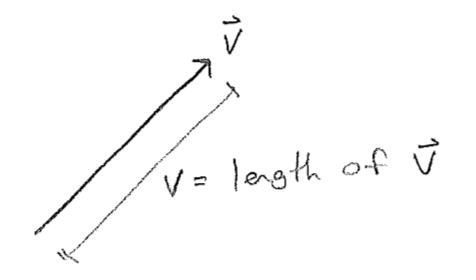
To be clear about notation, \(v\) is the length (norm) of a vector, more rigorously written as \(|\vec{v}|\), as reflected in the figure [#] below. We will often use this convention to declutter the appearance of equations.
Now we turn to the more subtle topic of potential energy. First, an observation: if a particle is subject to a field of forces that depend only on its position (and not otherwise on time or its velocity, etc.), then the following integral around a closed loop is zero.
\[
0 = \oint_{\substack{\vec{r}\text{ along} \\ \text{a closed path}}} \vec{F}(\vec{r}) \cdot \text{d}\vec{r}
\]
This "zero" has a simple geometric interpretation. If you travel in a closed loop in hilly terrain, you must climb up the same amount of elevation as you descend to return to your original location. Consider furthermore that all of your ascents and descents are accompanied by backward and forward forces, respectively, which impede and aid your progress. By the time the loop is complete, you will have experienced the same total amount of force in the forward and backward directions. In other words, these forces sum/integrate to zero over the journey. The integral above formalizes and generalizes this concept, where the dot product serves to extract the component of the force along the integration path. If the forces impinging on a particle obey this integral, then they can be described as the slope (gradient) of some scalar function \(V(\vec{r})\), which can be conceptualized as the elevation of hilly terrain. Formally, the relationship between \(\vec{F}\) and \(V\) is
\[\begin{align}
\vec{F}(\vec{r}) &= -\vec{\nabla} V(\vec{r}) \\
&=-\left(\begin{array}{l}
\frac{\partial}{\partial x} V(\vec{r}) \\
\frac{\partial}{\partial y} V(\vec{r}) \\
\frac{\partial}{\partial z} V(\vec{r}) \\
\end{array}\right)
\text{,}\end{align}\]
where we have introduced the gradient notation \(\vec{\nabla}\) for differentiation with respect to the components of \(\vec{r}\). The meaning of \(\vec{\nabla}\) is defined by the second line, presuming that \(\vec{r} = (x, y, z)\). For reasons, that will become clear soon, \(V\) is called a potential.
We are now in a position to write one of the grandest observations in physics. For a particle moving in a force field such as just described (say planet orbiting a star)
\[
E_\text{total}(t) ~=~ E_\text{kinetic}(t) + E_\text{potential}(t) ~=~ \text{constant}
\text{,}\]
where the definition of \(E_\text{potential}\) is via the time-dependent position as
\[
E_\text{potential}(t) = V\big(\vec{r}(t)\big)
\text{.}\]
Returning to the example of billiard balls, at the moment of a collision, two balls may appear to have stopped. At such time, the kinetic energy is suddenly decreased. However, if we consider that some energy is associated with the potential energy of the balls, due to the mutual forces compressing them, we would see that the total energy of the system (kinetic+potential) is a always conserved. Notably, since the potential \(V\) appears both in the definition of the potential energy and the definition of the forces that drive changes in velocities (and therefore kinetic energy), this exact trade-off between kinetic and potential energy only works when the "\(1/2\)" is present in the definition of \(E_\text{kinetic}\) in eq. \ref{classicalkinetic}.
c. Hamilton's equations and energy conservation
Now let us see how Hamilton's equations can be used to show that classical mechanics ensures energy conservation. For ease, let us consider a single particle in one dimension and suppress the vector hats. Realizing that we may make the substitution \(mv^2 = p^2/m\), we have for the total energy \(E\) (kinetic+potential)
\[
E(p,r) =\frac{1}{2 m} p^{2}+V(r)
\text{.}\]
We then can write
\[\begin{align}
\frac{\partial E(p,r)}{\partial p} &= \frac{1}{2m} 2p + 0 = \frac{1}{m} p \\
\frac{\partial E(p,r)}{\partial r} &= 0 + \frac{\partial V(r)}{\partial r} = -F(r)
\text{,}\end{align}\]
and Hamilton's equations (eqs. \ref{HamiltonR} and \ref{HamiltonP}) become abstractly
\[\begin{eqnarray}
\frac{\text{d}}{\text{d} t} r(t) &= \frac{1}{m} p(t) \; = &\frac{\partial E(p(t),r(t))}{\partial p} \\
\frac{\text{d}}{\text{d} t} p(t) &= F(t) \; =-&\frac{\partial E(p(t),r(t))}{\partial r}
\text{.}\end{eqnarray}\]
Remember have only rewritten Newton's equation using some definitions of energy that were observationally motivated. A simple application of calculus (suppressing some functional dependencies to reduce clutter) now gives
\[\begin{align}
\frac{d E}{d t} &=\frac{\partial E}{\partial p} \frac{d p}{d t} + \frac{\partial E}{\partial r} \frac{d r}{d t} \\
&=-\frac{\partial E}{\partial p} \frac{\partial E}{\partial r} + \frac{\partial E}{\partial r} \frac{\partial E}{\partial p} = 0
\text{.}\end{align}\]
This shows that the energy does not change with time. In other words, it is conserved. Since Newton's and Hamilton's equations are equivalent, energy conservation is a guaranteed feature of Newtonian mechanics as well. However, Hamiltonian mechanics makes this more obvious, in addition to having provided us with a notion of an instantaneous state that completely determines the system trajectory.
We will later see that energy is also a conserved quantity in quantum mechanics, under the same assumption that forces depend only on particle positions. If we are yet more restrictive and insist that that the potential energy of a system depends only on interparticle coordinates, we can also show that total momentum (the sum of all the particle momenta) is similarly conserved. The reason for bringing this up is to elevate the notion of momentum in the reader's mind. Although velocity is more directly observed, momentum is more fundamental. This will also be more obvious in quantum mechanics, beyond the mere aesthetic elegance it brings to Hamilton's formulation of classical mechanics. It would be good to get used to the idea that having a velocity (that is, moving between locations with time) is a consequence of having momentum, rather than the other way around.
2. Waves
a. mathematical description
Many things in nature are describable in terms of waves. For a traveling wave \(f\) in one dimension, the most basic equation is
\[
f(r, t) = A \sin \left(\frac{2 \pi}{\lambda}(r-vt)+\phi\right)
\text{,}\]
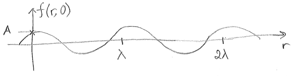
where \(r\) is the position coordinate over which the wave extends, \(t\) is time, \(v\) is the velocity of the wave, \(\lambda\) is its wavelength, \(A\) is its amplitude, and \(\phi\) is an arbitrary constant. Consider that, for \(t=0\),
\[
f(r, 0)=A \sin \left(2 \pi \frac{r}{\lambda}+\phi\right)
\text{,}\]
as shown in the above figure [#]. As can be seen in this figure, whenever \(r\) is an integer multiple of \(\lambda\), then \(f(r, 0)\) returns to the value \(f(0,0)\). The phase \(\phi\) simply accounts for the fact that, at \(r=0\), the wave may start at at any point within the wave cycle. As time advances, the whole wave travels forward, and any point (such as the one marked with an \(\times\) on the figure [#]) advances with velocity \(v\). An observer at a specific point \(r^\prime\) will see the wave return to its original value at intervals related to velocity and wavelength, obtained by solving the following equation for \(\Delta t\).
\[
A \sin \left(\frac{2\pi}{\lambda}(r^\prime-v(t+\Delta t))+\phi\right) = A \sin \left(\frac{2\pi}{\lambda}(r^\prime-v t)+\phi\right)
\]
This equation is solved whenever \(\Delta t\) is an integer multiple of \(T=\lambda/v\), known as the period. So the velocity of the wave is intuitively related to the time needed for one wavelength to travel to an equivalent location as \(v=\lambda/T\). Writing this equation in terms of the frequency with which the wave returns to its original form, \(\nu=1/T\), we obtain
\[
v=\lambda \nu
\text{.}\]
Note the subtle distinction between the Greek letter \(\nu\) (nu) and the Latin letter \(v\). While this may seem bothersome at present, there are very few contexts going forward in which these two might easily be confused (we will mostly use this equation for light, whereby \(v\) is replaced with \(c\)).
It is now useful to introduce a couple of simplified variables to describe a traveling wave
\[\begin{align}
k &= \frac{2\pi}{\lambda} \\
\omega &= 2\pi\nu
\text{.}\end{align}\]
The quantities \(k\) and \(\omega\) are called the wavevector and angular velocity, respectively; the name wavevector will seem more sensible in 2D or 3D, but, in 1D, it is a single number. We now can write
\[
f(r, t)=A \sin (k r-\omega t+\phi)
\text{.}\]
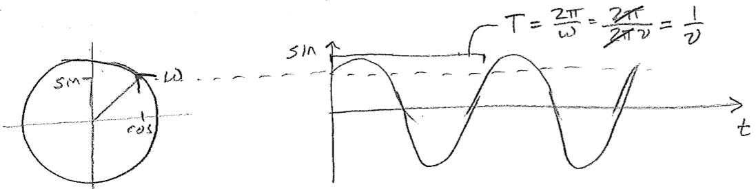
Note, just for entertainment, the strikingly similar way in which time and space appear in a traveling wave, this hints at the higher physics of wave mechanics in a relativistic framework, where space and time are not strictly distinct. Let us now give further interpretation to \(k\) and \(\omega\). The quantity \(\omega\) is clearly related to the frequency. It is called the angular velocity because of its relationship to an object proceeding in a circle. Since the object would complete one circuit for every \(2 \pi\) radians traveled, if its speed in radians per time is \(\omega\), then the frequency with which it comes back to the same position is \(\nu=\omega/(2 \pi)\), as illustrated in the figure [#] below. By analogy, \(k\) is proportional to the spatial frequency, or how many wave crests there are per distance (as opposed to time).
These variables of temporal and spatial frequency are particularly advantageous when dealing with multidimensional waves, which can be expressed, in 3D, for example, as
\[
f(\vec{r}, t)=A \sin (\vec{k} \cdot \vec{r}-\omega t+\phi)
\text{.}\]
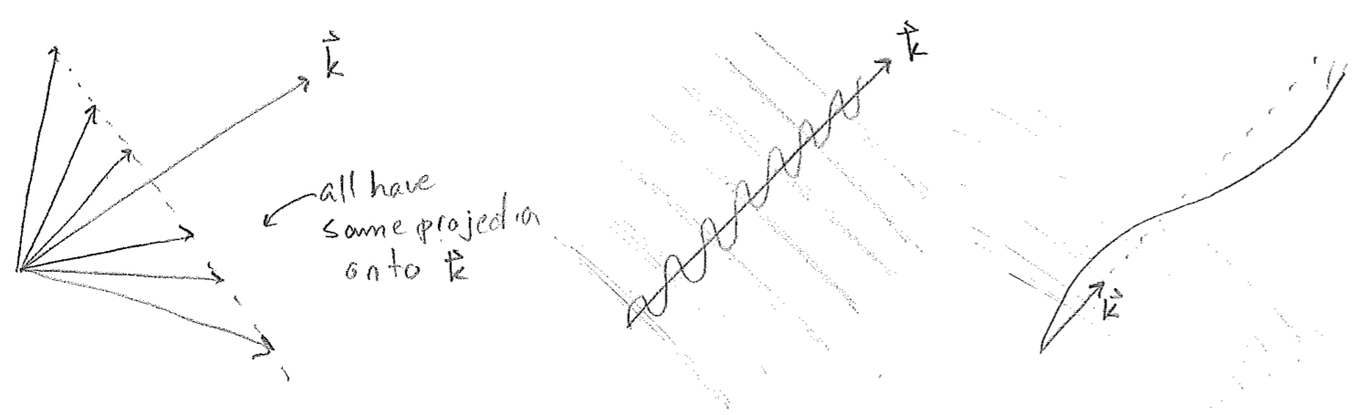
Whereas time is still a scalar, a point in space is now given by a vector \(\vec{r}\). The dot product takes the projection of \(\vec{r}\) onto a fixed vector \(\vec{k},\) which points in the direction of the wave, with a length proportional to spatial frequency, as illustrated in the figure [#] below. Such waves are called plane waves because, in 3D, the parallel wave fronts are arranged as a series of planes, though this terminology will also be used for such regular, infinitely repeating sinusoidal waves in 1D and 2D as well.
Another common description of waves is to use the raw frequency and the wavenumber, \(\bar{\nu}=1/\lambda\), to write, in 1D
\[
f(r, t) = A \sin (2 \pi(\bar{\nu} r-\nu t)+\phi)
\text{.}\]
We will prefer \(\bar{\nu}\) and \(\nu\), but not exclusively. Although this convention has some advantages, and is gaining in popularity, the use of \(k\) and \(\omega\) is still more common. It is still very uncommon, however, to write \(\vec{\bar{\nu}}\) for multidimensional waves, and the wavenumber \(\bar{\nu}\) is universally thought of as a scalar. In this text, we will also avoid promoting the wavenumber to a vector. When it is necessary, we will express this notion as \(\bar{\nu}\vec{u}\), where \(\vec{u}\) is a unit vector in the direction of travel.
b. wave properties
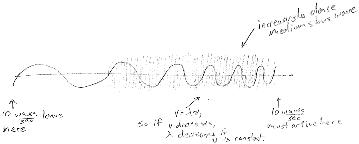
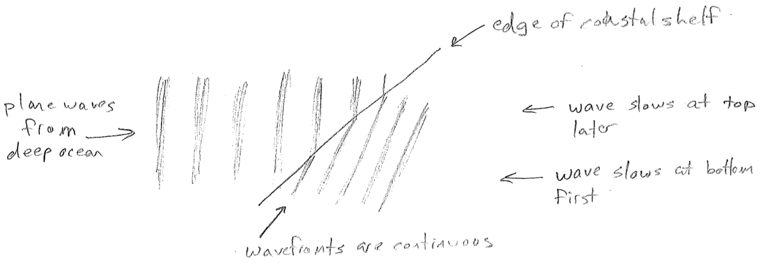
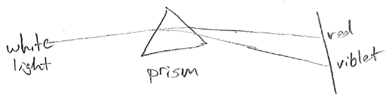
The equations presented so far are for idealized waves, without considering their sources or anything that may impede them. A real wave may, for example, change wavelength over space. One reason this can happen is that the source frequency might vary in time. Another very important reason is that the medium might cause the velocity to change, even though the frequency is constant, as illustrated in the figure [#] above. This slowing underlies the phenomenon of refraction. Consider a wave that suddenly changes velocity at a barrier, for example, waves on water that slow in shallow water, as shown in the figure [#] below. In order that wave crests and troughs are continuous, the wave must change direction at the boundary, producing shorter wavelengths. Refraction changing the direction of light is responsible for distortions when looking through a thick transparent object (like a glass of water) and underlies the notion of a lens. It is worthwhile to note that the change in velocity can depend on wavelength. Though the speed of light in vacuum is constant, in glass, blue light is slower than red. It therefore refracts more, leading to the prism effect, as shown in the figure [#] below.
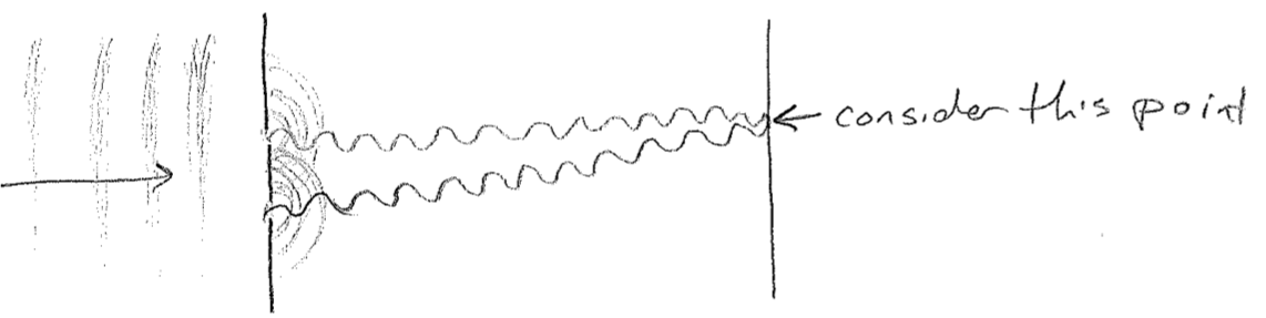
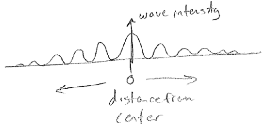
Another important aspect of waves is that they interfere, or diffract. The most famous example is a double-slit experiment, which can be done with waves on water. Plane waves are directed at a pair of slits. As the wave fronts exit the very small slits, they proceed away in all directions. As shown in the figure below [#], as the waves meet the screen on the other side, whether they are "up or down" at a given time depends on the number of wavelengths that can fit in the distance traveled. Consider then a fixed point on the screen; it will receive waves from both slits. If the distance to each slit is different by an integer multiple of wavelengths, then the waves from each source will be up or down at the same time, making a "wavy" spot on the screen. However, if the distances differ by a half-integer multiple, the level of the water at that point will be constant and calm because the two waves cancel exactly at all times. We call these two cases constructive and destructive interference, respectively. The intensity profile of the waves on the screen then will therefore show an alternating diffraction pattern of wavy and calm regions, as illustrated in the figure [#] below. In addition to water waves, light has been observed to diffract (giving rise to "wavy" bright spots and "calm" dark spots), convincing us unambiguously that light travels as a wave of some sort. Furthermore, diffraction patterns for electrons will be some of the most direct and powerful indicators of their wave nature.
A final facet of all waves is that they carry energy; it takes energy to produce them, and they can transfer that energy to other objects. In fact, waves can be considered to have (or be a form of) energy.
c. kinds of waves
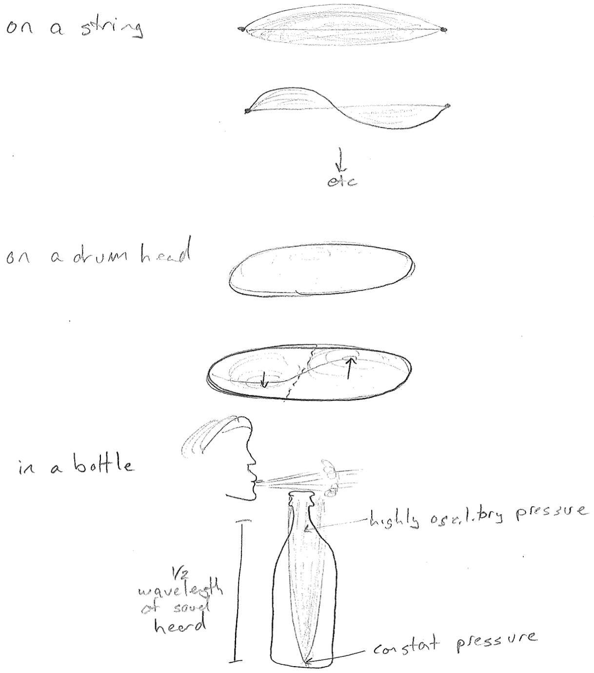
We have so far only eluded to the different kinds of waves. A wave is always described by a wave variable, something displaced from its average value. For example, the wave variable for an ocean wave is depth. On a string it is a displacement from a line. For sound it is pressure. See the figure [#] below for an illustration of each.

Finally, in addition to traveling waves, there may also be standing waves. As we will soon see, standing waves underlie the quantization in quantum mechanics. Standing waves oscillate in time, but the waveform does not change in space. In such a situation, time and space occur in separable functions.
\[
f(\vec{r}, t)=f_{0}(\vec{r}) \sin (2 \pi \nu t+\phi)
\]
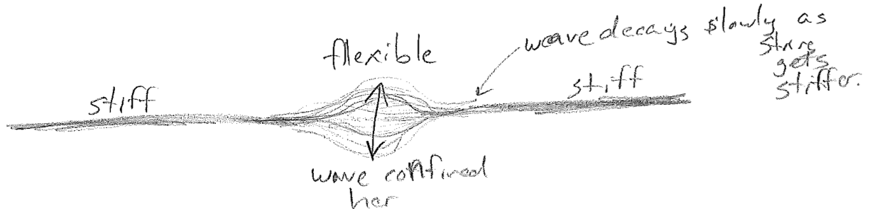
The spatial part has a constant shape, but its magnitude and sign oscillates in time uniformly across the spatial profile. Good examples of standing waves are on a string, on a drum head, and air in a bottle, as illustrated in the figure [#] above. It is worth noting that standing waves can also have non-sinusoidal spatial profiles. As an example, consider an oscillation on thin part of a stiff string, which is sinusoidal in time but not space, as illustrated in the figure [#] below.
3. Light as waves
Towards the end of the 1800s, James Clerk Maxwell united two fields, which had been separate until then. One field was the study of electricity and magnetism, and the other was optics, or the study of light. Through careful experimentation, he showed that electrically charged bodies and magnets (created by electrical currents) interacted with each other through time-dependent electric fields \(\vec{E}\) and magnetic fields \(\vec{H}\) that permeate space and obey the equations
\[\begin{align}
\vec{\nabla} \cdot \vec{E} &=\frac{\rho}{\varepsilon} & \frac{\partial \vec{E}}{\partial t} &= ~\frac{1}{\varepsilon}(\vec{J}+\vec{\nabla} \times \vec{H}) \\
\vec{\nabla} \cdot \vec{H} &=0 & \frac{\partial \vec{H}}{\partial t} &= -\frac{1}{\mu} \vec{\nabla} \times \vec{E}
\text{,}\end{align}\]
where \(\varepsilon\) and \(\mu\) are fundamental constants, and \(\rho\) and \(\vec{J}\) are charge and electrical current densities, respectively. Far away from any material objects, we have \(\rho=0\) and \(\vec{J}=0\), giving
\[
\vec{\nabla} \cdot \vec{E} = \vec{\nabla} \cdot \vec{H} = 0
\]
\[
\frac{\partial \vec{E}}{\partial t} = \frac{1}{\varepsilon} \vec{\nabla} \times \vec{H} \;\;\;\;\;\;\;\;
\frac{\partial \vec{H}}{\partial t} =-\frac{1}{\mu} \vec{\nabla} \times \vec{E}
\text{.}\]
Without going into details, observe how the dynamics (time derivatives) of each field \(\vec{E}\) and \(\vec{H}\) depends on the state of the other field, therefore coupling implicitly back to its own state. It is satisfying that this is reminiscent of the interplay between position and momentum in Hamilton's equations, though an exploration of this connection is beyond the scope of this text.
What Maxwell discovered is that, although \(\vec{E}\) and \(\vec{H}\) have charge and current densities as their sources, they travel through space as waves, waves that solve the particular set of equations shown above. It was beginning to be understood that these electromagnetic waves are light. For the record, \(c=1/\sqrt{\varepsilon \mu}\), lest the reader be concerned that the speed of light \(c\) has not made an appearance.
More precisely one should say that light is electromagnetic waves because what we call (visible) "light" is only the small fraction of the full range (or spectrum) of electromagnetic wavelengths. Electromagnetic waves in vacuum all have the speed, \(c \approx 3 \times 10^{8} \frac{m}{s},\), but wavelengths and frequencies can vary widely. Our eyes respond to wavelengths of 400 nm (purple) to 700 nm (red). The high-frequency jiggling of electrons in the sun sends out electromagnetic waves that bounce off of terrestrial objects and into our eyeballs. This causes ultrafast chemical reactions that detect the light, its frequency, and the direction from which it came, with our brains thereby constructing an image. Even higher frequencies of light, with sufficient exposure, can tear apart chemical bonds or remove electrons, doing damage to biomolecules, and causing cancer in organisms. These progressively higher frequencies are ultraviolet (non-ionizing), and x-ray and gamma radiation (ionizing). The slower motions of charges in warm objects (cooler than the sun or a light-bulb filament) radiate in the infrared and microwave regions. Infrared is useful for night vision, which "sees" heat. The common microwave oven is used for heating food by inducing water molecules to jiggle by "grabbing" onto the partial charges of the atoms. Even slower are radio waves, which will be discussed shortly.
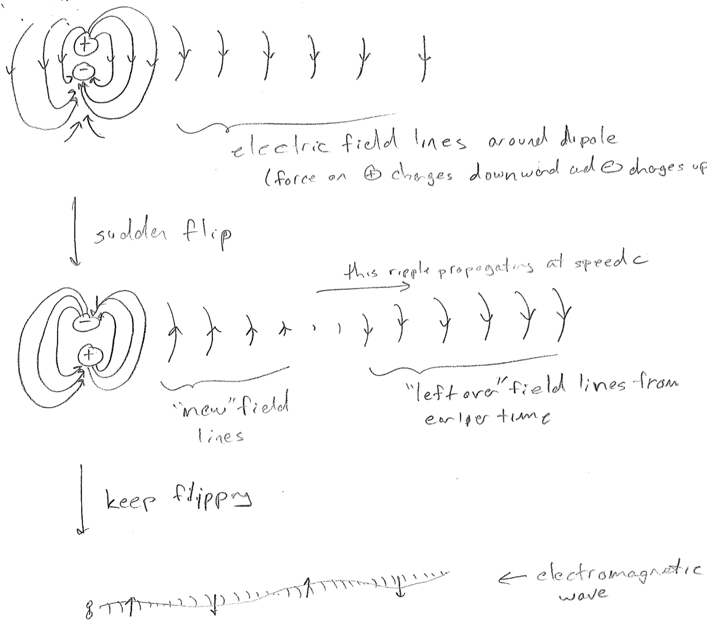
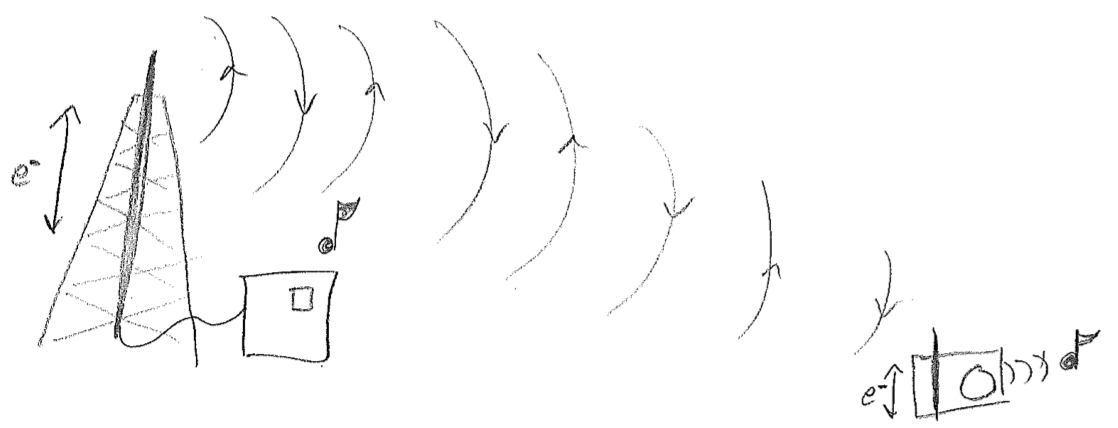
The simplest picture of electromagnetic radiation is the electric field emanating from an oscillating dipole, illustrated in the figure [#] above. What is clarified by this picture is that charged objects in a oscillating electromagnetic field will feel oscillatory pushes and pulls from the electric field. One of the most illustrative applications of electromagnetic dipolar radiation is at the longer wavelength (lower frequency) end of the spectrum. Radio waves oscillate so slowly (kHz to MHz) that we can control their waveforms with electronics. By shoving electrons back and forth along a wire, we create a custom oscillating field that can be detected and interpreted by another wire. Such wires are called antennas (transmission or receiving), and that is how a radio works, as shown in the figure [#] below.
4. The atom
a. evidence from chemistry
During the renaissance, Robert Boyle had already forwarded a rigorous definition of a chemical element as a substance that cannot be decomposed into other substances, and many elements had been isolated. But the microscopic (i.e., atomic) nature of these elements was still hidden from observation. By the early 1800s, three laws (summaries of observations) had been established concerning chemical reactions. These would eventually lead to theory that matter was composed of atoms.
- The law of mass conservation (Antoine Lavoisier): The products of a chemical reaction have the same total mass as the reactants, as long as they are completely captured.
- The law of definite proportion (Joseph-Louis Proust): In the preparation of a compound substance, regardless of the details of the synthesis, the same mass ratio of elements is incorporated into the compound.
- The law of multiple proportions (John Dalton): Elements may combine in different mass ratios to form different compounds.
Regarding the third law, certain regularities had been noticed, for example, \(\text{H}_{2} \text{O}_{2}\) requires precisely twice as much oxygen as \(\text{H}_{2} \text{O}\). The fact that this ratio is a simple integer is a clue about something deeper. This led John Dalton to propose the notion of atoms around the year 1800. These are indivisible and indisposable units of matter, whose rearrangements explain chemical reactions. Since atoms persist, mass is conserved. Arrangement into groups of integer numbers of atoms (i.e., molecules) explains the observed ratios, with these ratios defining the properties of compound substances.
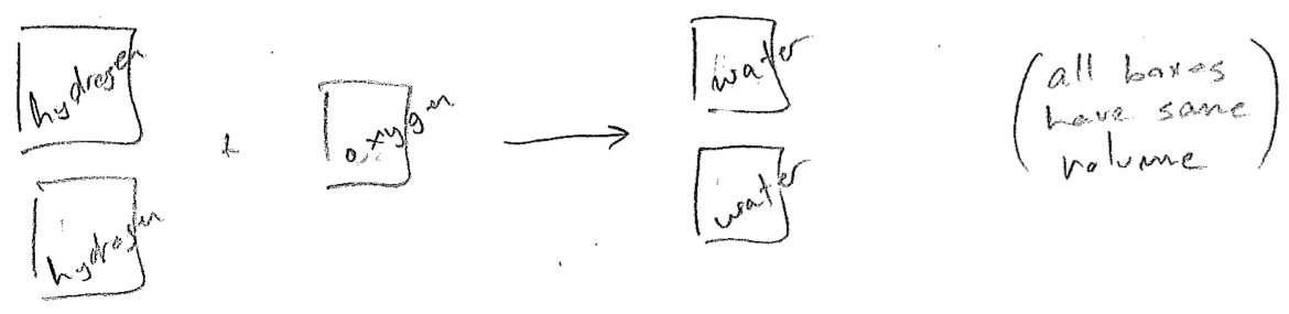
A researcher by the name of Joseph Gay-Lussac noted that, in some gas phase reactions, integer ratios of gas volumes were needed, as illustrated in the figure [#] below, for example. Building on a conjecture by Amedeo Avogadro, that a given volume of gas contains the same number af "molecules" (as asserted by Dalton's atomic theory), one then deduces that oxygen molecules must be \(\text{O}_{n}\), where \(n\) is an even integer because, otherwise, an O atom would be split between two water molecules (eventually, we know it is \(\text{O}_{2}\)). Through knowledge of many such processes, the formulas for the elements (e.g., \(\text{H}_{2}\), \(\text{O}_{2}\), \(\text{S}_{8}\), etc.) were discovered, and also molecular formulas of compounds. Simultaneously, the periodic table was emerging, even predicting new elements and inferring the relative masses of their atoms.
b. determining the constituents of matter
The indirectness of the chemists' inferences about atoms bothered physicists. For example, only relative masses could be established, e.g. \(\text{mass}_\text{C} \approx 12 \times \text{mass}_\text{H}\). Not until physicists could weigh atoms against the standard kilogram did they fully accept the atoms chemists had been using for 100 years by then. This was not until 1908, when Jean Baptiste Perrin confirmed a 1905 prediction by Einstein. Einstein's prediction applied Ludwig Boltzmann's statistical mechanics to Brownian motion. It was premised on the notion of atoms (which Boltzmann assumed must exist), but masses and numbers of collisions were independent parameters. This provided the first avenue for estimating atomic masses in terms of concrete units.
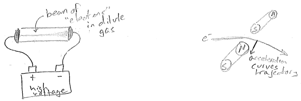
As physicists began to accept that atoms existed, they were also doing experiments that would further elucidate that atoms were not the smallest units of matter. In the late 1890s Joseph John Thomson had subjected gases to high voltages, as illustrated in the figure [#] below. At a high enough voltage, almost any dilute gas could be made to conduct electricity. Furthermore, it did so by creating a dramatic colored beam that connected the electrodes. Since the beam would deflect in a magnetic field, as expected from a charged body, it was concluded that matter consisted of separable charged particles and that electrical current (previously known but not understood) could be attributed to the motions of these particles. So atoms must consist of charged particles.
Remarkably, this explanation of moving charges being the basis of current was consistent with Maxwell's equations of electromagnetism (a moving charge should generate a magnetic field, and so should a current). The size of the beam deflection by the magnet is related to sideways acceleration of the particles, and acceleration is equal to force over mass by Newton's equation \((a=F/m)\). The force on a particle should also be proportional to its charge. Therefore, due to the fortuitous way that the unknown beam velocity cancels out in determining both force and acceleration, Thomson's experiment was able to provide the mass-to-charge ratio of the "electrons" (as they were called, due to their relationship to electricity). If one could determine either the charge or the mass, the other quantity would then be known.
In 1909, Robert Millikan's oil drop experiment provided the missing charge. Using drops of oil of a well-known density, he could determine the gravitational force acting on them, by measuring their size with a microscope. Simultaneously, he induced negative charges onto the droplets by exposing them to ionizing radiation. (In retrospect, we understand that electrons from ionized air were leaping onto the droplets, but Millikan only knew that the droplets became somehow negative, the same as Thomson's beam.) By adjusting the charges on plates above and below, the droplets could be made to levitate, as shown in the figure [#] below. By knowing the voltage and the force that must be being produced, he then could determine the charge on the droplet. His result was that the droplets differed in charge by integer multiples of some fundamental negative charge. This this must then be the charge of the electron. This led to a surprise when the absolute mass of a electron was compared to the absolute mass of an atom (recently available). The mass of an electron is tiny!
At this point, it is now understood that there are atoms, that atoms must consist of positive and negative charges, and that the negative charges have small mass. But how the charges are arranged in an atom is still a mystery.
c. problems with the internal structure of atoms
In 1911, Ernest Rutherford performed some of the first experiments that follow a paridigm still used today: shoot high energy particles at matter to look for clues about its internal structure. Through experiments similar to those on the electron, it had already become clear that \(\alpha\) radiation consists of positive particles much heavier than an electron. So if an \(\alpha\) particle and an electron collide, one expects very little deflection of the \(\alpha\)-particle. Therefore, when Rutherford shot a very fast \(\alpha\)-particle beam at a thin gold foil and observed a substantial backscatter, it was concluded that both positive charges (the \(\alpha\)-particle and that within the atom) must be very compact, in order to concentrate enough force to reverse the \(\alpha\)-particle trajectory. See the illustration in the figure [#] below. Combined with Millikan's result, we conclude that most of the mass of the atom is also be contained in this compact, positive "nucleus."
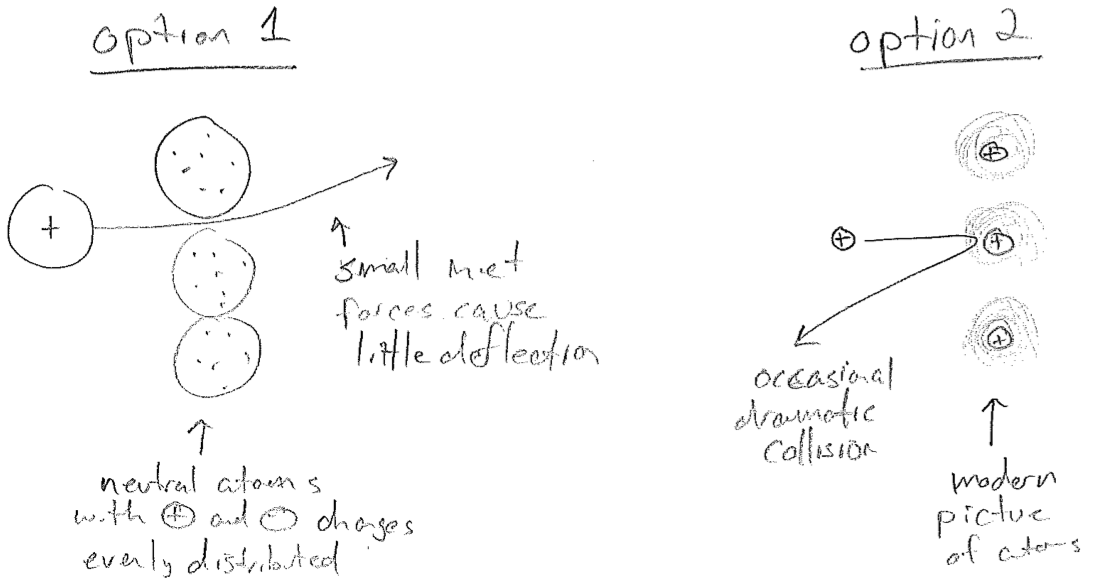
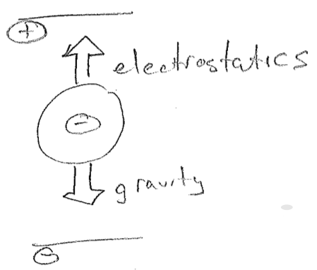
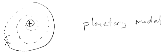
A picture of the inside of an atom was developing; light negative electrons orbit a heavy positive nucleus. This was a big problem. Recall from the above that an oscillating dipole emits light. Light carries energy. So the electrons in atoms will constantly lose energy, eventually crashing into the nucleus, as illustrated in the figure [#] below. Furthermore, if Coulomb's law for attracting charges,
\[
V(\vec{r}) \propto -\frac{1}{|\vec{r}|}
\text{,}\]
holds at such small distances, then there is a divergence in the potential energy as they get infinitesimally close; \(\vec{r}\) is the separation between the charges. Every atom would collapse, meanwhile releasing an infinite amount of light energy. Something was seriously wrong, something that will be resolved by quantum theory.
d. the mystery of atomic spectra
There was another mystery of the atom lurking in the background. Since 1814, spectral lines in light either emitted from or absorbed by matter had been quite a curiosity. (The word "line" refers to literal lines of brightness or darkness made on a screen after light is dispersed by a prism, in the event that only a few wavelengths are present or missing, respectively.) The first such discovery was by Joseph von Fraunhofer, of the eponymous Fraunhofer lines. He noted that certain specific colors of light were missing or weak, when coming from the sun.
Eventually, as it also came also to be understood that light is a wave, it came to be realized that the atmosphere is absorbing strongly at the missing Fraunhofer wavelengths. Also, as it came to be understood that matter is made of atoms, it was observed that heated atoms in gases give a spectrum of discrete lines that is characteristic of their element type. Furthermore, the wavelengths absorbed by a certain atom are also among the wavelengths emitted when heated, as seen in the figure [#] below. By 1900, the empirical relationship between spectrum and element type was already a powerful analytical technique for composition analysis (for which the chemists Robert Bunsen and Gustav Kirchhoff are known); helium in the sun was discovered first by its spectrum. Today, this technique is incredibly quantitative.
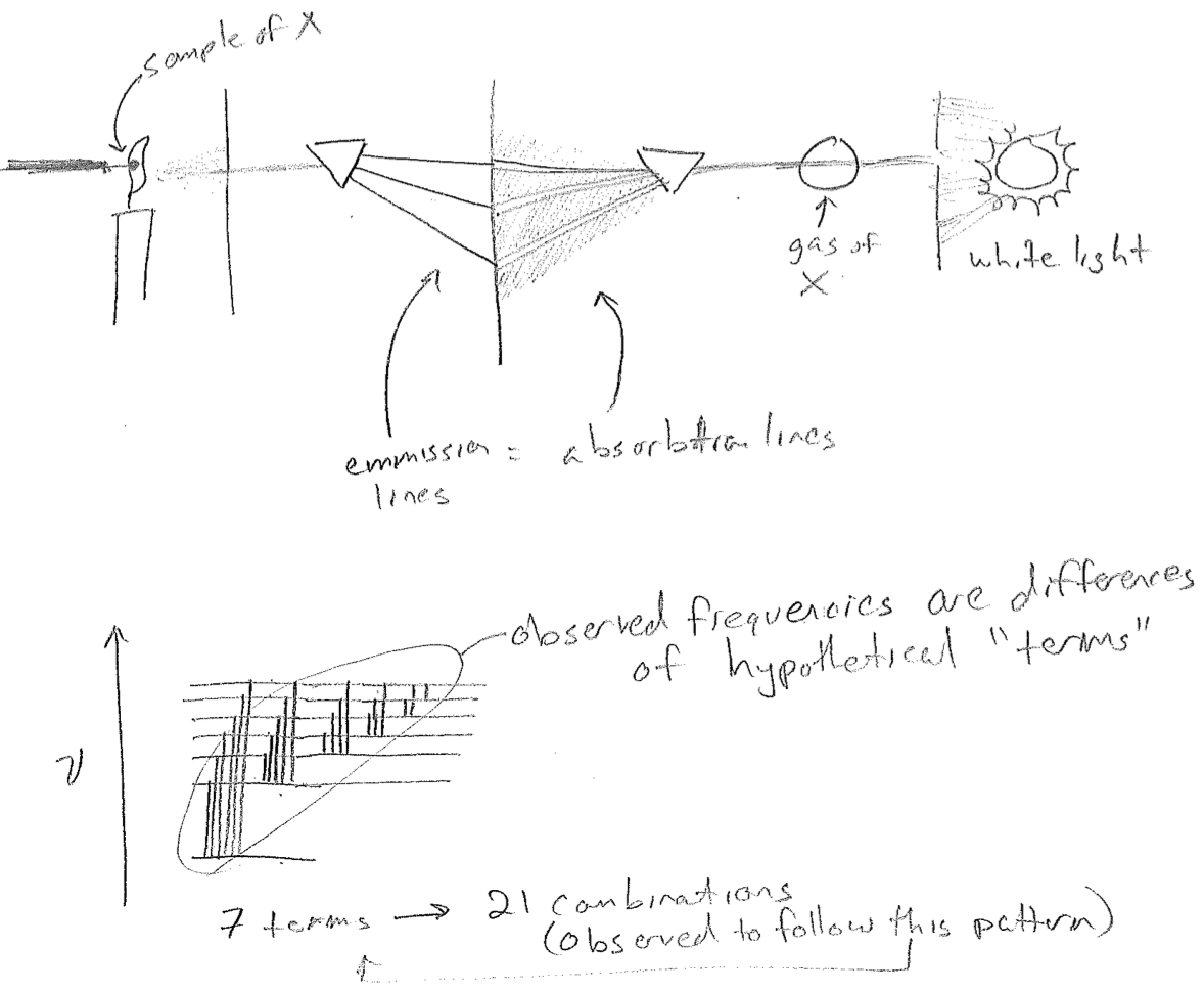
The final aspect of this mystery was again one of uncanny regularity. According to the combination principle framed by Walter Ritz in 1908, the spectrum of any atom could be explained by sums and differences of a smaller number of "terms," as if the different frequencies were connecting levels on some abstract chart, as illustrated in the figure [#] above. In particular, it was known that the terms \(T_n\) for the hydrogen atom obey the expression
\[
T_n = \frac{109678 \, \text{cm}^{-1}}{n^{2}} \label{Hterms}
\text{,}\]
where \(n\) is an integer. Differences of these terms are directly the wavenumbers of the light absorbed or emitted by hydrogen atoms, according to
\[
\bar{\nu}_{mn} = T_m - T_n
\text{,}\]
for \(m<n\). These wavenumbers are directly proportional to frequency and can easily be converted to wavelength, but older literature (and much modern literature) still prefers wavenumbers, due to a direct connection to the measurement process of using diffraction gratings (sold with a certain number of grating lines per cm). Note that the discussion above can easily be adapted to include a negative sign in the numerator of eq. \ref{Hterms}, which better fits its later quantum interpretation in terms of energy.