6.5: Bonding and Antibonding Orbitals

The two molecular orbitals created via the linear combinations of atomic orbitals (LCAOs) approximation were created from the sum and the difference of two atomic orbitals. Within this approximation, the j^th molecular orbital can be expressed as a linear combination of many atomic orbitals {\(\phi_i\)}:

\[\psi_J  = \sum_i^N c_{J,i}   \phi_i  \label{1}\]

A molecule will have as many molecular orbitals as there are atomic orbitals used in the basis set (\(N\) in Equation \(\ref{1}\)). Adding two atomic orbitals corresponds to constructive interference between two waves, thus reinforcing their intensity; the internuclear electron probability density is increased. The molecular orbital corresponding to the sum of the two H 1s orbitals is called a σ_1s combination (parts (a) and (b) of Figure \(\PageIndex{1}\)).

Figure \(\PageIndex{1}\): Molecular Orbitals for the \(H_2\) Molecule. (a) This diagram shows the formation of a bonding \(σ_{1s}\) molecular orbital for \(H_2\) as the sum of the wave functions (\(Ψ\)) of two H 1s atomic orbitals. (b) This plot of the square of the wave function (\(Ψ^2\)) for the bonding σ1s molecular orbital illustrates the increased electron probability density between the two hydrogen nuclei. (Recall that the probability density is proportional to the square of the wave function.) (c) This diagram shows the formation of an antibonding \( \sigma _{1s}^{*} \) molecular orbital for \(H_2\) as the difference of the atomic orbital wavefunctions (\(Ψ\)) of two H 1s atomic orbitals. (d) This plot of the square of the wave function (Ψ2) for the \( \sigma _{1s}^{*} \) antibonding molecular orbital illustrates the node corresponding to zero electron probability density between the two hydrogen nuclei. Image used with permission (CC BY-SA-NC; anonymous by request).

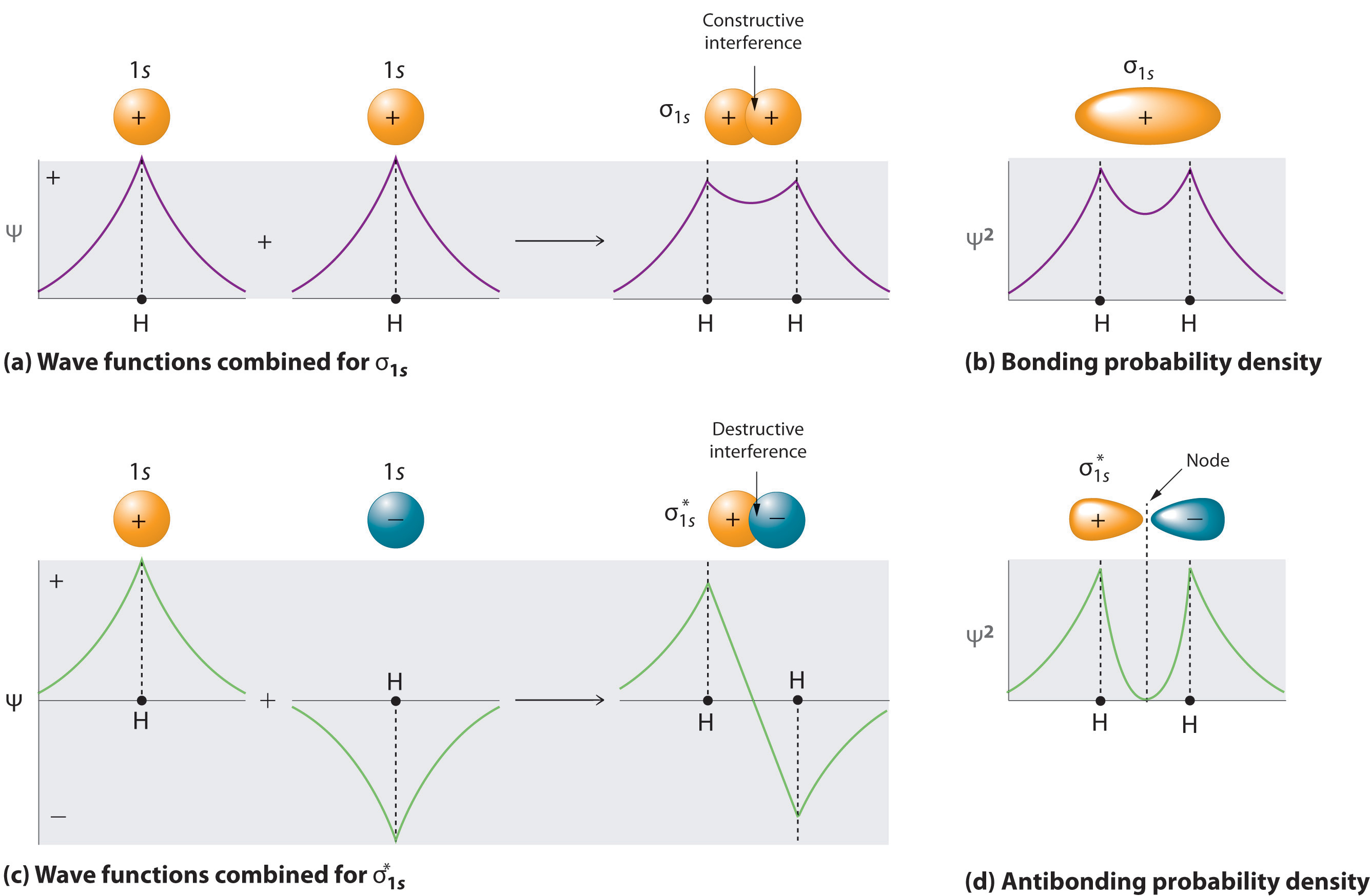
In the sigma (\(σ\)) orbital, the electron density along the internuclear axis and between the nuclei has cylindrical symmetry; that is, all cross-sections perpendicular to the internuclear axis are circles. The subscript 1s denotes the atomic orbitals from which the molecular orbital was derived.

\[ \sigma _{1s} = \dfrac{1}{\sqrt{2(1 + S )}} \left(  1s_A  + 1s_B  \right) \label{2} \]

Conversely, subtracting one atomic orbital from another corresponds to destructive interference between two waves, which reduces their intensity and causes a decrease in the internuclear electron probability density (part (c) and part (d) in Figure \(\PageIndex{1}\)). The resulting pattern contains a node where the electron density is zero. The molecular orbital corresponding to the difference is called \( \sigma _{1s}^{*} \) and has a region of zero electron probability, a nodal plane, perpendicular to the internuclear axis:

\[  \sigma _{1s}^*  = \dfrac{1}{\sqrt{2(1 - S )}} \left( 1s_A -  1s_B  \right) \label{3} \]

The electron density in the σ_1s molecular orbital is greatest between the two positively charged nuclei, and the resulting electron–nucleus electrostatic attractions reduce repulsions between the nuclei. Thus the σ_1s orbital represents a bonding molecular orbital. A molecular orbital that forms when atomic orbitals or orbital lobes with the same sign interact to give increased electron probability between the nuclei due to constructive reinforcement of the wave functions. In contrast, electrons in the \( \sigma _{1s}^{\star } \) orbital are generally found in the space outside the internuclear region. Because this allows the positively charged nuclei to repel one another, the \( \sigma _{1s}^{\star } \) orbital is an antibonding molecular orbital (a molecular orbital that forms when atomic orbitals or orbital lobes of opposite sign interact to give decreased electron probability between the nuclei due to destructive reinforcement of the wave functions).

Note

Antibonding orbitals contain a node perpendicular to the internuclear axis; bonding orbitals do notal is always lower in energy (more stable) than the component atomic orbitals, whereas an antibonding molecular orbital is always higher in energy (less stable).

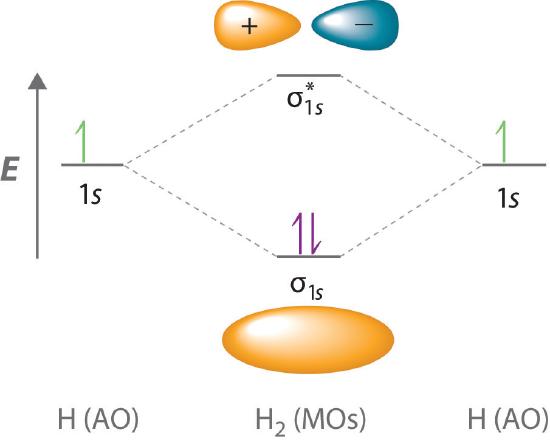
Because electrons in the σ_1s orbital interact simultaneously with both nuclei, they have a lower energy than electrons that interact with only one nucleus. This means that the σ_1s molecular orbital has a lower energy than either of the hydrogen 1s atomic orbitals. Conversely, electrons in the \( \sigma _{1s}^{\star } \) orbital interact with only one hydrogen nucleus at a time. In addition, they are farther away from the nucleus than they were in the parent hydrogen 1s atomic orbitals. Consequently, the \( \sigma _{1s}^{\star } \) molecular orbital has a higher energy than either of the hydrogen 1s atomic orbitals. The σ_1s (bonding) molecular orbital is stabilized relative to the 1s atomic orbitals, and the \( \sigma _{1s}^{\star } \) (antibonding) molecular orbital is destabilized. The relative energy levels of these orbitals are shown in the energy-level diagram (a schematic drawing that compares the energies of the molecular orbitals (bonding, antibonding, and nonbonding) with the energies of the parent atomic orbitals) in Figure \(\PageIndex{2}\)

Figure \(\PageIndex{2}\): Molecular Orbital Energy-Level Diagram for H2. The two available electrons (one from each H atom) in this diagram fill the bonding σ1s molecular orbital. Because the energy of the σ1s molecular orbital is lower than that of the two H 1s atomic orbitals, the H2 molecule is more stable (at a lower energy) than the two isolated H atoms.

Note

A bonding molecular orbital is always lower in energy (more stable) than the component atomic orbitals, whereas an antibonding molecular orbital is always higher in energy (less stable).

 

Contributors and Attributions

• David M. Hanson, Erica Harvey, Robert Sweeney, Theresa Julia Zielinski ("Quantum States of Atoms and Molecules")

• Modified by Valeria D. Kleiman