2.4: Operators, Observables and Wavefunctions

What are Operators?

Operators are rules to convert a function or number into another a function or number. Operators are symbolized by a ^ above a letter.

The symbol +represents the operator sum , which takes 2 numbers and adds them together, the symbol \( \cdot\) corresponds to the operator multiplication, which multiplies two numbers or functions together to obtain a new number or new function. Other examples of operators are

• Differentiation = \( \textcolor{purple}{\hat{D} =\dfrac{d}{dx}}\) applied to the function \(f(x) \) yields the derivative of that function

\[ \textcolor{purple}{\dfrac{d}{dx}}f(x) = \frac{df(x)}{dx}= f'(x)\]

\[ \textcolor{purple}{\hat{D}^2= \dfrac{d^2}{dx^2}}f(x) = \textcolor{purple}{\frac{d}{dx}}\frac{df(x)}{dx}= f"(x)\]

• Multiplication This operator multiplies a number or a function to another function

\[ \textcolor{purple}{\hat{x}} f(x)= \textcolor{purple}{x\cdot }{f(x)} =xf(x) \hspace{1cm}\text{or} \hspace{1cm}\textcolor{purple}{3\cdot f(x)}=3f(x)\]

In Quantum Mechanics, operators are used to write the Schrödinger equation for a particle-wave.

Example \(\PageIndex{1}\)

What is the result of applying the operator \(\textcolor{purple}{\dfrac{d}{dx}}\) to the function \( f(x) = 4x^3-22x\)

Solution

\(\textcolor{purple}{\dfrac{d}{dx}} f(x) =\textcolor{purple}{\dfrac{d}{dx}} (4x^3-22x )= \dfrac{d(4x^3-22x)}{dx}=\dfrac{d(4x^3)}{dx}-\dfrac{d(22x)}{dx} = 3\cdot 4x^2-22 = 12x^2-22\)

Observables

In Quantum Mechanics, each observable property (something that we can measure in the lab, like the energy, the momentum, the position, etc) has a corresponding operator.

Energy

If we want to measure the energy of a particle, we look for the corresponding operator, that is the Hamiltonian, \( \textcolor{purple}{\hat{H}}\)

The Hamiltonian \( \textcolor{purple}{\hat{H}}\) has two components,, one associated with kinetic energy \( \textcolor{purple}{\hat{T}}\) and one associated with potential energy \( \textcolor{purple}{\hat{V}}\) .

\[ \textcolor{purple}{\hat{H} = \hat{T}+ \hat{V}} \]

For a particle-wave that is moving in one-dimension,\( \ \textcolor{purple}{\hat{T}= -\dfrac{\hbar^2}{2m}\dfrac{d^2}{dx^2}}\). If the particle is moving in 3-dimensions, the operator associated with the Kinetic Energy becomes

\[ \textcolor{purple}{\hat{T}} = - \dfrac{\hbar^2}{2m}\cdot  \left( \dfrac{d^2}{dx^2}+\dfrac{d^2}{dy^2}+\dfrac{d^2}{dz^2} \right)\]

The operator associated with Potential Energy will depend on each specific system (whether the system is rotating or oscillating, or whether it includes 1, 2 or multiple particles, etc). For each system there will be a specific \( \textcolor{purple}{\hat{V}}\) that will be use to describe the particular conditions of the particle-wave, thus for each specific system there is a particular Hamiltonian.

For each system there is one specific Schrödinger equation where we apply the Hamiltonian operator to the function of the wave and obtain as a result the energy of the system. \[\textcolor{purple}{\hat{H}} \psi(x) = \textcolor{darkgreen}{E}\cdot \psi(x) \label{1}\]

Equation \ref{1} is a differential equation, and quantum mechanics is devoted to find the functions that are proper solutions to this differential equation. This means to find the functions \(\psi(x)\) that when we apply the Hamiltonian to it, we obtain a number E corresponding to the energy, multiplied by the same function \(\psi (x)\).

Since for each Hamiltonian, there are always an infinite number of \(\psi(x)\) and E solutions, each pair corresponds to a state of the system (ground state, excited state 1 excited state 2, etc) and is identified by its quantum numbers.

Momentum

If we want to measure the momentum of a particle, we look for the corresponding operator, that is the momentum operator, \( \textcolor{purple}{\hat{p}}\) .

The momentum operator is given by \( \textcolor{purple}{\hat{P}=-i \hbar\dfrac{d}{dx}}\)

There is an equivalent equation for the momentum \[\textcolor{purple}{\hat{P}} \psi(x) = \textcolor{darkgreen}{p}\cdot \psi(x)\] where p corresponds to the numerical value of the momentum that we would measure in the lab if the system is found in a state described by the wavefucntion \( \psi(x)\).

Wavefunctions

Although this time-independent Schrödinger Equation can be useful to describe a matter wave in free space, we are most interested in waves when confined to a small region, such as an electron confined in a small region around the nucleus of an atom. Several different models have been developed that provide a means by which to study a matter-wave when confined to a small region: the particle in a box (infinite well), the Hydrogen atom, molecules. We will discuss each of these in order to develop a greater understanding for how a wave behaves when it is in a bound state.

Figure \(\PageIndex{1}\) : Two unacceptable wavefunctions. (left) This is not a single-valued function and (right) this is a non-continuous function

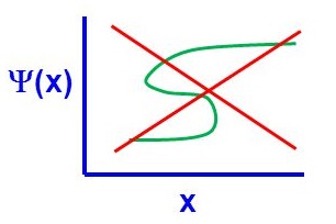
There are four general aspects that are applicable to an acceptable wavefunction

1. An acceptable wavefunction will be the solution of the Schrödinger equation (either Equations \(\ref{1}\)).
2. An acceptable wavefunction must be normalizable so will approaches zero as position approaches infinity.
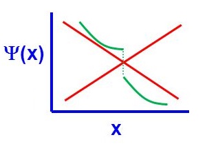
3. An acceptable wavefunction must be a continuous function of position.
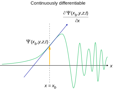
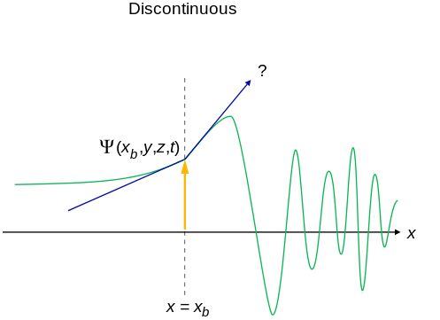
4. An acceptable wavefunction will have a continuous slope (Figure \(\PageIndex{2}\)).

Figure \(\PageIndex{2}\):Wavefunction continuity in space.

Interpretation

As we saw before, the physical significance cannot be found from the function itself, instead the absolute square of the wavefunction, which also is called the square of the modulus is used.

\[ {|\psi (r , t ) |}^2 \]

where \(r\) is a vector (x, y, z) specifying a point in three-dimensional space. The square is used, rather than the modulus itself, just like the intensity of a light wave depends on the square of the electric field. At one time it was thought that for an electron described by the wavefunction \(\psi(r)\), the quantity \(e\psi^*(r_­i)\psi(r_i)d\tau\) was the amount of charge to be found in the volume \(d\tau\) located at \(r_i\). However, Max Born found this interpretation to be inconsistent with the results of experiments.

The Born interpretation, which generally is accepted today, is that \(|\psi (r , t ) |^2\ d\tau\) is the probability that the electron is in the volume \( d\tau \) located at \(r_i\) at time \(t \). The Born interpretation therefore calls the wavefunction the probability amplitude, the absolute square of the wavefunction is called the probability density, and the probability density times a volume element in three-dimensional space (\(d\tau\)) is the probability.

Normalization

A probability is a real number between 0 and 1. An outcome of a measurement which has a probability 0 is an impossible outcome, whereas an outcome which has a probability 1 is a certain outcome. The probability of a measurement of \(x\) yielding a result between \(-\infty\) and \(+\infty\) is

\[P_{x \in -\infty:\infty} = \int_{-\infty}^{\infty}\vert\psi(x)\vert^{ 2} dx. \label{3.6.2}\]

However, a measurement of \(x\) must yield a value between \(-\infty\) and \(+\infty\), since the particle has to be located somewhere. It follows that \(P_{x \in -\infty:\infty}(t) =1\), or

\[\int_{-\infty}^{\infty}\vert\psi(x)\vert^{ 2} dx = 1, \label{3.6.3}\]

which is generally known as the normalization condition for the wavefunction.

Summary

For each observable property, we can construct an equation that will connect the operator to the wavefunction describing the specific state of a system. When studying a quantum mechanical system, we start a problem by finding the Hamiltonian that describes the system, and then we look for all the possible wavefunctions \(\psi(x)\) that can solve Equation \ref{1}. Each solution corresponds to one state of the system.

Contributions and Attributions

• Valeria D. Kleiman
• The wavefunction section is from David M. Hanson, Erica Harvey, Robert Sweeney, Theresa Julia Zielinski ("Quantum States of Atoms and Molecules")