
6: Determination of Kc for a Complex Ion Formation (Experiment)
- Page ID
- 126995
Objectives
- Find the value of the equilibrium constant for the formation of \(\ce{FeSCN^{2+}}\) by using the visible light absorption of the complex ion.
- Confirm the stoichiometry of the reaction.
In the study of chemical reactions, chemistry students first study reactions that go to completion. Inherent in these familiar problems—such as calculation of theoretical yield, limiting reactant, and percent yield—is the assumption that the reaction can consume all of one or more reactants to produce products. In fact, most reactions do not behave this way. Instead, reactions reach a state where, after mixing the reactants, a stable mixture of reactants and products is produced. This mixture is called the equilibrium state; at this point, a chemical reaction occurs in both directions at equal rates. Therefore, once the equilibrium state has been reached, no further change occurs in the concentrations of reactants and products.
The equilibrium constant, \(K\), is used to quantify the equilibrium state. The expression for the equilibrium constant for a reaction is determined by examining the balanced chemical equation. For a reaction involving aqueous reactants and products, the equilibrium constant is expressed as a ratio between reactant and product concentrations, where each term is raised to the power of its reaction coefficient (Equation \ref{1}). When an equilibrium constant is expressed in terms of molar concentrations, the equilibrium constant is referred to as \(K_{c}\). The value of this constant at equilibrium is always the same, regardless of the initial reaction concentrations. At a given temperature, whether the reactants are mixed in their exact stoichiometric ratios or one reactant is initially present in large excess, the ratio described by the equilibrium constant expression will be achieved once the reaction composition stops changing.
\[a \text{A} (aq) + b\text{B} (aq) \ce{<=>}c\text{C} (aq) + d\text{D} (aq) \]
with \[ K_{c}= \frac{[\text{C}]^{c}[\text{D}]^{d}}{[\text{A}]^{a}[\text{B}]^{b}} \label{1}\]
We will be studying the reaction that forms the reddish-orange iron (III) thiocyanate complex ion, \(\ce{Fe(H2O)5SCN^{2+}}\) (Equation \ref{2}). The actual reaction involves the displacement of a water ligand by thiocyanate ligand, \(\ce{SCN^{-}}\) and is often call a ligand exchange reaction.
\[\ce{Fe(H2O)6^{3+} (aq) + SCN^{-} (aq) <=> Fe(H2O)5SCN^{2+} (aq) + H2O (l)} \label{2}\]
For simplicity, and because water ligands do not change the net charge of the species, water can be omitted from the formulas of \(\ce{Fe(H2O)6^{3+}}\) and \(\ce{Fe(H2O)5SCN^{2+}}\); thus \(\ce{Fe(H2O)6^{3+}}\) is usually written as \(\ce{Fe^{3+}}\) and \(\ce{Fe(H2O)5SCN^{2+}}\) is written as \(\ce{FeSCN^{2+}}\) (Equation \ref{3}). Also, because the concentration of liquid water is essentially unchanged in an aqueous solution, we can write a simpler expression for \(K_{c}\) that expresses the equilibrium condition only in terms of species with variable concentrations.
\[\ce{Fe^{3+} (aq) + SCN^{-} (aq) <=> FeSCN^{2+} (aq)} \label{3}\]
In this experiment, students will create several different aqueous mixtures of \(\ce{Fe^{3+}}\) and \(\ce{SCN^{-}}\). Since this reaction reaches equilibrium nearly instantly, these mixtures turn reddish-orange very quickly due to the formation of the product \(\ce{FeSCN^{2+}}\) (aq). The intensity of the color of the mixtures is proportional to the concentration of product formed at equilibrium. As long as all mixtures are measured at the same temperature, the ratio described in Equation \ref{3} will be the same.
Measurement of [\(\ce{FeSCN^{2+}}\)]
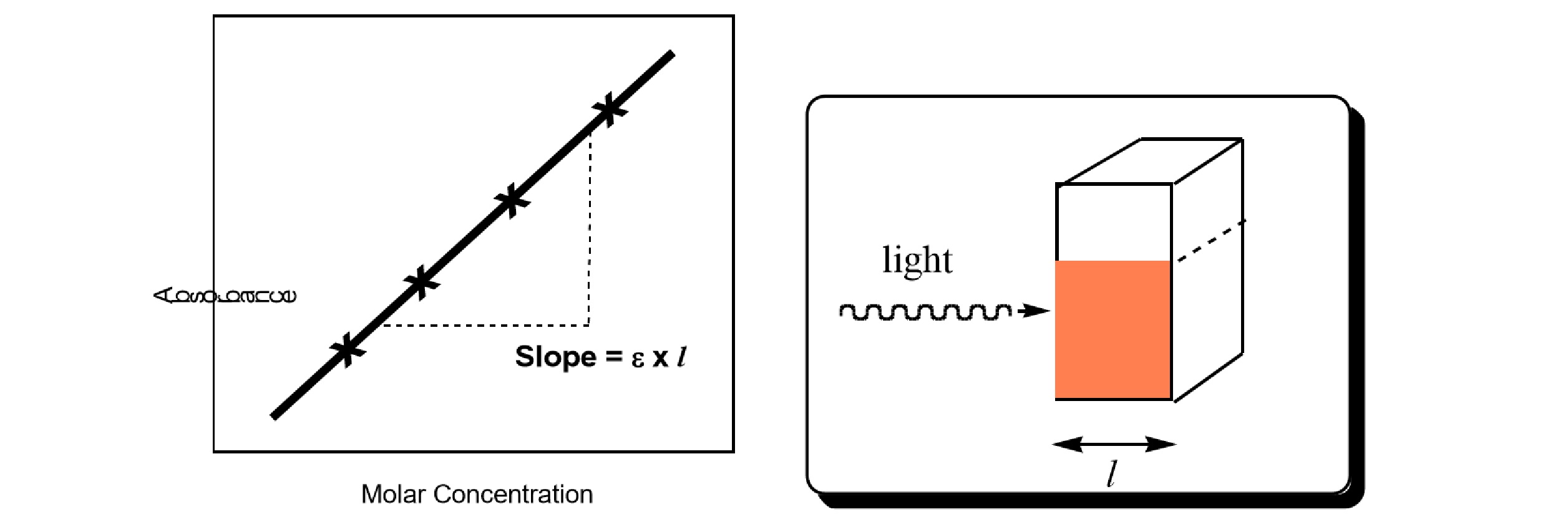
Since the complex ion product is the only strongly colored species in the system, its concentration can be determined by measuring the intensity of the orange color in equilibrium systems of these ions. Two methods (visual inspection and spectrophotometry) can be employed to measure the equilibrium molar concentration of \(\ce{FeSCN^{2+}}\), as described in the Procedure section. Your instructor will tell you which method to use. Both methods rely on Beer's Law (Equation \ref{4}). The absorbance, \(A\), is directly proportional to two parameters: \(c\) (the compound's molar concentration) and path length, \(l\) (the length of the sample through which the light travels). Molar absorptivity \(\varepsilon\), is a constant that expresses the absorbing ability of a chemical species at a certain wavelength. The absorbance, \(A\), is roughly correlated with the color intensity observed visually; the more intense the color, the larger the absorbance.
\[A=\varepsilon \times l \times c \label{4}\]
In the visual inspection method, you will match the color of two solutions with different concentrations of \(\ce{FeSCN^{2+}}\) by changing the depth of the solutions in a vial. As pictured in Figure \(\PageIndex{1}\), the solution on the left is more concentrated than the one on the right. However, when viewed from directly above, their colors can be made to "match" by decreasing the depth of the more concentrated solution. When the colors appear the same from above, the absorbances, \(A\), for each solution are the same; however, their concentrations and path lengths are not.
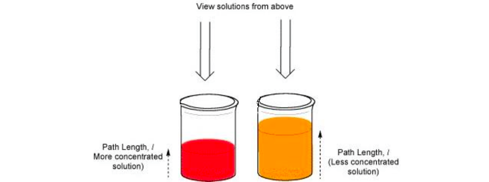
If a standard sample with a known concentration of \(\ce{FeSCN^{2+}}\) is created, measurement of the two path lengths for the "matched" solutions allows for the calculation of the molar concentration of \(\ce{FeSCN^{2+}}\) in any mixture containing that species (Equation \ref{5}). This equation is an application of Beer's Law, where \(\frac{A}{\varepsilon}\) for matched samples are equal. Therefore, the product of the path length, \(l\), and molar concentration, \(c\), for each sample are equal.
\[l_{1} \times c_{1} = l_{2} \times c_{2} \label{5}\]
By using a spectrophotometer, the absorbance, \(A\), of a solution can also be measured directly. Solutions containing \(\ce{FeSCN^{2+}}\) are placed into the spectrophotometer, and their absorbances at 447 nm are measured. In this method, the path length, \(l\), is the same for all measurements. Rearrangement of Equation \ref{4} allows for the calculation of the molar concentration, \(c\), from the known value of the constant \(\varepsilon \times l\). The value of this constant is determined by plotting the absorbances, \(A\), vs. molar concentrations, \(c\), for several solutions with known concentration of \(\ce{FeSCN^{2+}}\) ( Figure \(\PageIndex{2}\)). The slope of this calibration curve is then used to find unknown concentrations of \(\ce{FeSCN^{2+}}\) from their measured absorbances.
Calculations
In order to determine the value of \(K_{c}\), the equilibrium values of \([\ce{Fe^{3+}}]\), \([\ce{SCN^{–}}]\), and \([\ce{FeSCN^{2+}}]\) must be known. The equilibrium value of \([\ce{FeSCN^{2+}}]\) was determined by one of the two methods described previously; its initial value was zero, since no \(\ce{FeSCN^{2+}}\) was added to the solution.
The equilibrium values of \([\ce{Fe^{3+}}]\) and \([\ce{SCN^{-}}]\) can be determined from a reaction table ('ICE' table) as shown in Table \(\PageIndex{1}\). The initial concentrations of the reactants—that is, \([\ce{Fe^{3+}}]\) and \([\ce{SCN^{-}}]\) prior to any reaction—can be found by a dilution calculation based on the values from Table \(\PageIndex{2}\) found in the procedure. Once the reaction reaches equilibrium, we assume that the reaction has shifted forward by an amount, \(x\). The equilibrium concentrations of the reactants, \(\ce{Fe^{3+}}\) and \(\ce{SCN^{-}}\), are found by subtracting the equilibrium \([\ce{FeSCN^{2+}}]\) from the initial values. Once all the equilibrium values are known, they can be applied to Equation \ref{3} to determine the value of \(K_{c}\).
| Reaction \ref{3} | \(\ce{Fe^{3+}}\) | \(\ce{+\quad SCN^{-}}\) | \(\ce{<=> FeSCN^{2+}}\) |
|---|---|---|---|
| Initial Concentration | \([\ce{Fe^{3+}}]_{i}\) | \([\ce{+ SCN^{-}}]_{i}\) | 0 |
| Change in Concentration | \(- x\) | \(- x\) | \(+ x\) |
| Equilibrium Concentration | \([\ce{Fe^{3+}}]_{i} - x\) | \([\ce{+ SCN^{-}}]_{i} - x\) | \(x= [\ce{FeSCN^{2+}}]\) |
The reaction "ICE" table demonstrates the method used in order to find the equilibrium concentrations of each species. The values that come directly from the experimental procedure are found in the shaded regions. From these values, the remainder of the table can be completed.
Standard Solutions of \(\ce{FeSCN^{2+}}\)
In order to find the equilibrium \([\ce{FeSCN^{2+}}]\), both methods require the preparation of standard solutions with known \([\ce{FeSCN^{2+}}]\). These are prepared by mixing a small amount of dilute \(ce{KSCN}\) solution with a more concentrated solution of \(ce{Fe(NO3)3}\). The solution has an overwhelming excess of \(\ce{Fe^{3+}}\), driving the equilibrium position far towards products. As a result, the equilibrium \([\ce{Fe^{3+}}]\) is very high due to its large excess, and therefore the equilibrium \([\ce{SCN^{-}}]\) must be very small. In other words, we can assume that ~100% of the \(\ce{SCN^{-}}\) is reacted, meaning that \(\ce{SCN^{-}}\) is a limiting reactant resulting in the production of an equal amount of \(\ce{FeSCN^{2+}}\) product. Examine the Kc-expression to prove this to yourself. In summary, due to the large excess of \(\ce{Fe^{3+}}\), the equilibrium concentration of \(\ce{FeSCN^{2+}}\) can be approximated as the initial concentration of \(\ce{SCN^{-}}\).
Procedure
Materials and Equipment
Solutions: Iron(III) nitrate (2.00 x 10⁻³ M) in 1 M \(\ce{HNO3}\); Iron(III) nitrate (0.200 M) in 1 M \(\ce{HNO3}\); Potassium thiocyanate (2.00 x 10⁻³ M).
Materials:
50-mL beaker x 2, Test tubes, stirring rod, 1-mL and 2-mL volumetric pipet, 5-mL and 10-mL volumetric pipet*, 10- mL graduated cylinder, Pasteur pipets, spectrometers, and cuvets* (2).
*must obtain from stockroom
Safety
The iron(III) nitrate solutions contain nitric acid. Avoid contact with skin and eyes; wash hands frequently during the lab and wash hands and all glassware thoroughly after the experiment. Collect all your solutions during the lab and dispose of them in the proper waste container.
Part A: Solution Preparation
Label two clean, dry 50-mL beakers, and pour 30 mL of 2.00 x 10⁻³ M \(\ce{Fe(NO3)3}\) (already dissolved by the stockroom in 1 M \(\ce{HNO3}\)) into one beaker. Then pour 20 mL of 2.00 x 10⁻³ M \(\ce{KSCN}\) into the other beaker. At your work area, label five clean and dry medium test tubes to be used for the five test mixtures you will make. Using your volumetric pipet, add 5.00 mL of your 2.00 x 10⁻³ M \(\ce{Fe(NO3)3}\) solution into each of the five test tubes. Next, using your 1-mL and 2-mL volumetric pipet, add the correct amount of \(\ce{KSCN}\) solution to each of the labeled test tubes, according to the table below. Rinse out your volumetric pipet with deionized water, and then use it to add the appropriate amount of deionized water into each of the labeled test tubes. Stir each solution thoroughly with your stirring rod until a uniform orange color is obtained. To avoid contaminating the solutions, rinse and dry your stirring rod after stirring each solution.
| Mixture | \(\ce{Fe(NO3)3}\) Solution | \(\ce{KSCN}\) Solution | Water |
|---|---|---|---|
| 1 | 5.00 mL | 5.00 mL | 0.00 mL |
| 2 | 5.00 mL | 4.00 mL | 1.00 mL |
| 3 | 5.00 mL | 3.00 mL | 2.00 mL |
| 4 | 5.00 mL | 2.00 mL | 3.00 mL |
| 5 | 5.00 mL | 1.00 mL | 4.00 mL |
Five solutions will be prepared from 2.00 x 10⁻³ M \(\ce{KSCN}\) and 2.00 x 10⁻³ M \(\ce{Fe(NO3)3}\) according to this table. Note that the total volume for each mixture is 10.00 mL, assuming volumes are additive. If the mixtures are prepared properly, the solutions will gradually become lighter in color from the first to the fifth mixture. Use this table to perform dilution calculations to find the initial reactant concentrations to use in Figure \(\PageIndex{3}\).
Part B:
1. Preparation of a Standard Solution of \(\ce{FeSCN^{2+}}\)
Before examining the five test mixtures, prepare a standard solution with a known concentration of \(\ce{FeSCN^{2+}}\). Obtain 15 mL of 0.200 M \(\ce{Fe(NO3)3}\). (Note the different concentrations of this solution.) Rinse your volumetric pipet with a few mL of this solution, and add 10.00 mL of this solution into a clean and dry large test tube. Using your graduated cylinder, add 8.00 mL deionized water to the large test tube. Rinse your volumetric pipet with a few mL of 2.00 x 10⁻³ M \(\ce{KSCN}\). Then add 2.00 mL of the \(\ce{KSCN}\) solution to the large test tube. Mix the solution with a clean and dry stirring rod until a uniform dark-orange solution is obtained. This solution should be darker than any of the other five solutions prepared previously.
2. Spectrophotometric Determination of \([\ce{FeSCN^{2+}}]\)
Your instructor may ask you to measure the absorbance of each test mixture using a spectrophotometer rather than by matching the colors with a standard solution. In this case, you will be creating a calibration curve that plots the absorbance of \(\ce{FeSCN^{2+}}\) at 447 nm vs. molar concentration. From this curve, you can determine \([\ce{FeSCN^{2+}}]\) in each mixture from the absorbance at 447 nm.
A few dilutions of the standard solution prepared in Part B1 will be used to prepare four standard solutions for your calibration curve. In addition, one 'blank' solution containing only \(\ce{Fe(NO3)3}\) will be used to zero the spectrophotometer. The instructor will decide if each group of students will work alone or with other groups to prepare the standards. Table \(\PageIndex{3}\) shows the preparation method for each of the standards.
| Tube | Composition |
|---|---|
| Blank | 0.200 M \(\ce{Fe(NO3)3}\) in 1 M \(\ce{HNO3}\) (Stock Solution Part B) |
| 1 | Standard Solution (Part B) |
| 2 | 4.00 mL Standard Solution + 1.00 mL \(\ce{H2O}\) |
| 3 | 4.00 mL Standard Solution + 2.00 mL \(\ce{H2O}\) |
| 4 | 4.00 mL Standard Solution + 3.00 mL \(\ce{H2O}\) |
Four standard solutions and one blank solution will be prepared for the calibration curve. Your instructor will tell you if you need to create all these solutions or if groups can share solutions.
Fill a cuvet with the blank solution and carefully wipe off the outside with a tissue. Insert the cuvet and make sure it is oriented correctly by aligning the mark on the cuvet towards the front. Close the lid. Your instructor will show you how to zero the spectrophotometer with this solution. Set aside this solution for later disposal. For each standard solution in Table \(\PageIndex{3}\), rinse your cuvet three times with a small amount (~0.5 mL) of the standard solution to be measured; dispose of the rinse solution each time. Then fill the cuvet with the standard, insert the cuvet as before and record the absorbance reading. Finally, repeat this same procedure with five mixtures with unknown \([\ce{FeSCN^{2+}}]\) prepared in Part A, Table \(\PageIndex{2}\) . The \([\ce{FeSCN^{2+}}]\) in this solutions will be read from the calibration curve.