Lab 4: Molecular Fluorescence

goals

1. Students should have an in-depth understanding of fluorescence after the completion of this lab exercise.
2. Students should be able to optimize the scan parameters to achieve the best emission and excitation spectra.
3. Students should be able to extract key information from the emission and excitation spectra and determine the unknown concentration of a compound.

Introduction

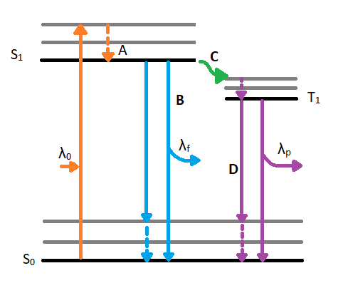
When a molecule absorbs a photon in the ultraviolet or visible (UV VIS) region (180 - 780 nm), an electronic transition occurs within the molecule. This transition involves moving an electron from the singlet ground state to a singlet excited state. After excitation, the molecule will undergo de-excitation to regain its ground state electronic configuration. De-excitation of the molecule can occur in three distinct ways: by collisional deactivation (external conversion), fluorescence, or phosphorescence (Figure 4.1).

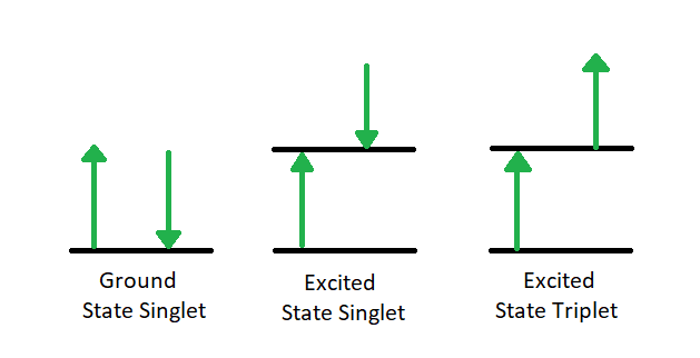
The first relaxation mechanism, collisional deactivation, occurs when the excited molecule transfers its excess energy to molecules with which it collides without photon emission. The second mechanism, fluorescence, involves the electron returning from the excited singlet state to the ground singlet state accompanied by the emission of a photon of lower energy (longer wavelength) than the absorbed photon; the energy loss is due to vibrational relaxation while in the excited state. When fluorescence is favored, it occurs within about 10^-8 seconds after absorption. For reference, a picosecond is 10^-9 seconds. Phosphorescence, the third route for de-excitation, occurs when the excited electron enters the lowest triplet state from the excited singlet state by intersystem crossing and subsequently emits a photon in returning from the lowest triplet state to the singlet ground state. These excited singlet-triplet and triplet- ground singlet transitions involve electron reversal (Figure 4.2), which is a low probability occurrence. Thus, the time between absorption and phosphorescence can be from 10^-2 seconds to several minutes.

Figure 4.1: Jablonski diagram displaying excitation and de-excitation pathways of a molecule. λ₀ indicates the incident wavelength that is absorbed by the molecule. Once the molecule reached the excited singlet state (S1) from the ground state singlet (S₀), is can experience vibrational relaxation as seen in A. After relaxing to the lowest energy excited state, a molecule can de-excited by fluorescence as seen in path B. The fluorescence path emits a wavelength (λf) which is longer than the absorbed wavelength (λ0). The alternative, unfavored path moves along path C which involves intersystem crossing. Intersystem crossing involves a conversion from an excited singlet state(S1) to an excited triplet state (T1). After reaching the triplet state and experiencing vibrational relaxing, the molecule will phosphoresce by emitting an even shorter wavelength (λp) to reach the ground state singlet (S₀).

Figure 4.2: Transition from Ground Singlet (A) to Excited Singlet (B) to Excited Triplet (C).

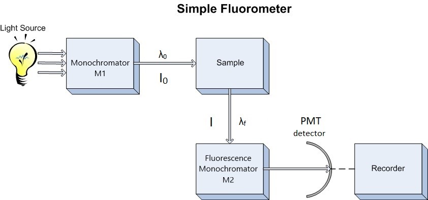
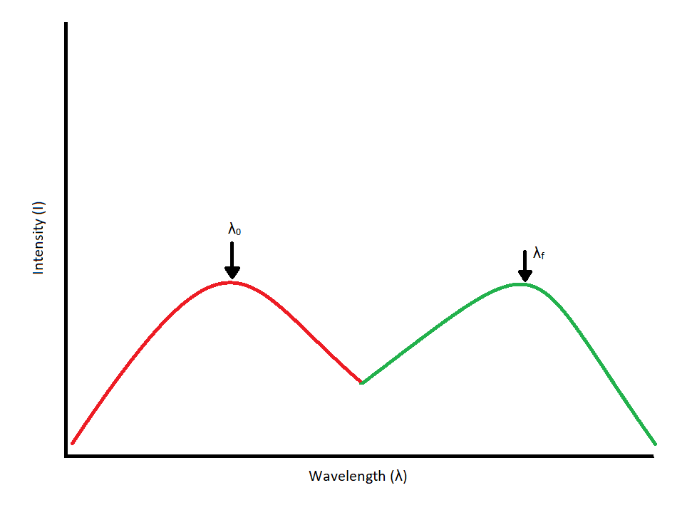
Since our interest involves fluorescence, a typical experimental arrangement is shown in Figure 4.3. This is used in either of two distinct ways. The first, which holds the excitation monochromator M1 fixed, and varies the emission monochromator M2, yields an emission spectrum (the wavelength distribution of light emitted by the excited singlet state). When generating an emission section, the intensity of the transmitted light (I) is measured and compared to the transmitted light's measured wavelength (λ_f). Alternately, M2 can be fixed and M1 varied; this procedure produces an excitation spectrum (a plot of fluorescence intensity as a function of excitation wavelength). The excitation spectrum can be produced by measuring the intensity of the transmitted light (I) and comparing it to the measured wavelength of the incident light (λ₀). Often, the excitation spectrum of a pure compound has exactly the same profile as the absorption spectrum (Figure 4.1). The principles described by Figure 4.1 can be observed in the excitation and emission spectra. An example of these spectra can be seen in Figure 4.4.

Figure 4.3: Schematic Diagram of Fluorometer. M1 = excitation monochromator, M2 emission monochromator, Photo Multiplier Tube detector.

Figure 4.4: Excitation/Absorbance Spectrum (Red) coupled with an emission spectrum (Green). Each spectrum peaks at its respective wavelength. Excitation and emission spectra should overlap and be mirror images of each other.

Coupling the above techniques with a relationship between fluorescence intensity and concentration would be exceptionally useful. Such a relationship can be derived from Beer's Law, which states that the fraction of light intensity transmitted by a sample is

\[\dfrac{I}{I_o} = 10^{-\epsilon b c} \label{4.1}\]

where,

• I is the transmitted light intensity,
• I₀ is the incident intensity,
• ε is the molar absorptivity at a given wavelength in units of L*mol^-1*cm^-1,
• b is the cell path in centimeters, and
• c is the concentration in moles per liter.

The fraction of absorbed light is: \[1 - \dfrac{I}{I_o} = 1 - 10^{-\epsilon b c} \label{2}\]

from which it follows that the absolute amount of absorbed light is equal to: \[I_o - I = I_o - I_o \left(10^{-\epsilon b c} \right) \label{3}\]

The fluorescence intensity, F, is proportional to the amount of light absorbed and fluorescence quantum yield, Φ. Thus, \[F = kI_o \phi \left[1-\left(10^{-\epsilon bc} \right) \right] \label{4}\]

where \(k\) is a proportionality constant. If dilute solutions are used, so that less than 2% of the excitation energy is absorbed, the exponential term in Equation \(\ref{4}\) can be approximated by the first two terms in the corresponding Taylor series expansion

\[e^x \approx 1 + x\]

Then, \[F = kI_o \phi \epsilon bc \label{5}\]

hence fluorescence intensity is proportional to concentration, but only at low concentration:

\[F \propto c \]

Instrumentation

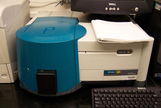
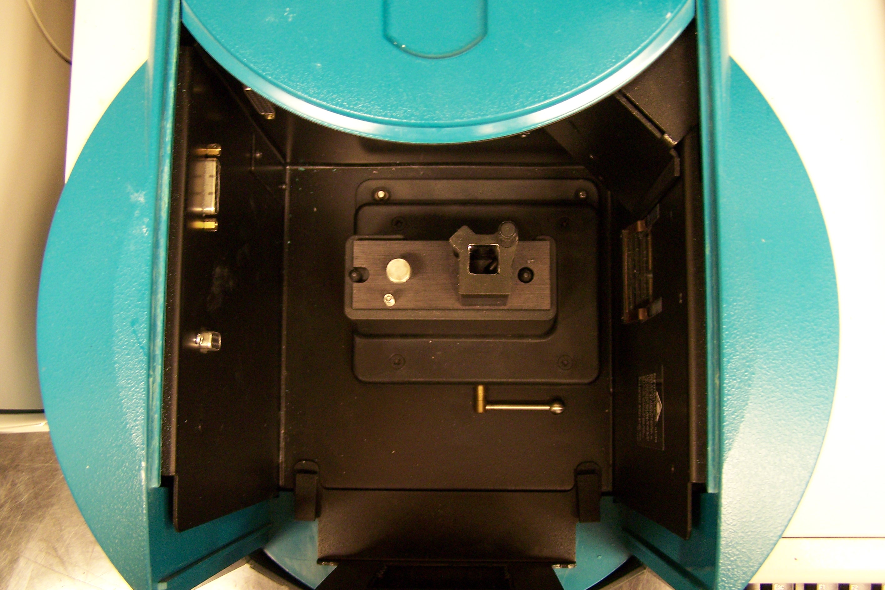
In this experiment, two instruments will be used. First, the Agilent HP8453 UV-Vis spectrometer to measure optimal excitation wavelength. You used this instrument in CHE 105, so you may remember how to use it. For the second portion of this experiment, the Varian Eclipse Fluorescence Spectrometer (Figure 4.5) will be used. This instrument is computer-controlled through software running on Windows XP. Detailed operating instructions for the Eclipse will be in the procedure section.

Figure 4.5: UCD's Varian Eclipse Fluorescence Spectrometer

Experimental Procedure

This experiment involves the analysis of vitamin B₂, riboflavin, by measuring its native fluorescence. Riboflavin (Figure 4.6) is a common water-soluble vitamin found in eggs, milk, and other foods, that strongly fluoresces and is very sensitive to light. Its two predominant irradiation decomposition products are lumichrome and lumiflavin, which are themselves highly fluorescent.

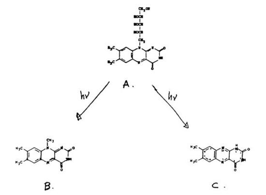
Figure 4.6: Riboflavin (A) and the two most predominant irradiation decomposition products, lumiflavin (B) and lumichrome (C).

The analysis method requires working with riboflavin samples at concentrations well below the part per million (ppm) level. Therefore, it is extremely important that the utmost care is exercised in cleaning and handling all of the glassware and solutions during this experiment.

In the first lab period, the standard and unknown solutions mentioned below should be prepared. Later during this period, you should consult the T.A. about operating the UV VIS spectrophotometer as well as the fluorescence spectrometer. You should also obtain the absorption spectra of riboflavin and perform a practice run on the fluorescence spectrometer.

The second lab period should be used to complete the experiment and Part II of the unknown analysis.

Stock Solutions

1. Obtain the 100 ppm stock standard solution of Riboflavin from the refrigerator or from the T.A.
2. Allow the solution to sit on the counter for a few minutes to equilibrate to room temperature. This is to ensure consistent volume measurements.
3. Deliver 1 mL of the stock solution to a 10 mL volumetric flask and dilute using deionized water. This is your 10 ppm solution.
4. Using a volumetric pipet, deliver 1.00 mL of the 10 ppm solution to a 100 mL volumetric flask, and dilute using deionized water. This is your 100 part per billion (ppb) stock solution.
5. Fill in Table 4.1 with the correct amounts of 100 ppb riboflavin to make the remainder of your standards. Check the table with your TA before you begin the experiment.
6. Make the solutions 2-6 from the table and dilute with deionized water. Make certain that your glassware is clean and rinsed with deionized water.

Table 4.1: Standard Riboflavin Solutions

Solution #	mL of 100 ppb sol.	Dilute to (mL)	Rib. Conc (ppb)
2		50	2
3		50	10
4		50	20
5		50	40
6		50	50

Unknown Solution

The dry milk sample should be reconstituted as indicated on the jar. Record your work (this is a quantitative experiment). The milk samples require special treatment in order to remove interfering fats and proteins, which would otherwise make analysis difficult or impossible. The procedure to accomplish this is outlined below.

1. Find the dry milk sample on the shelves above the weigh station.
2. Reconstitute the dry milk sample by following the directions listed on the sample jar.
3. Take 25 mL of milk sample and add exactly 75 mL of a solution consisting of equal parts 3M HAc and 3M NaCl. Do not use a volumetric flask for this. It is too difficult to stir the solution. Use your 25 mL pipet and a 250 or 400 mL beaker.
4. Stir for 20 minutes.
5. Filter the solution using a Buchner funnel and the vacuum line. Make sure you have a trap between the filtering flask and the house vacuum line.
6. Take a 5 mL aliquot of the filtrate and dilute to 100 mL with deionized water in a volumetric flask. This solution will be used for your analytical measurements.

Instrumental

Part 1: Approximate Excitation Wavelength

The instrument you'll be using in this portion of the experiment is an Agilent HP8453 UV-Vis spectrometer.

The first step in conducting the analysis is to determine the optimum excitation wavelength for riboflavin. When no prior information is available, as in this case, the absorption spectrum can be used to approximate the best excitation wavelength.

Look near the Agilent HP8453 UV-Vis spectrometer for a pack of cuvettes. If you cannot find a pack, ask your T.A. for a new pack. Use the 10 ppm solution to obtain an absorption spectrum of riboflavin from 280 to 600 nm. Use distilled water as your reference solution. If you do not recall how to acquire an absorbance spectrum, check with your TA for instructions. The wavelength of maximum absorbance should be used as an initial excitation wavelength. There may be more than one absorbance peak.

*Print the absorbance spectrum*

Part 2: Actual Excitation and Emission Maxima

In this part of the experiment, you will determine the optimal instrument operation parameters. Using the approximate excitation wavelengths determined above from the UV-Vis absorbance spectrum, obtain two emission spectra. The emission maximum observed in the two emission spectra will then be used to collect an excitation spectrum to "refine" the choice of excitation wavelength. You will see that the fluorescence excitation spectrum closely follows the absorbance spectrum.

You should collect the following spectra:

1. Two emission spectra of the 50 ppb standard solution will be taken. Collect the first spectrum from the first excitation wavelength (~370 to 700 nm). Collect the second spectrum from the second excitation wavelength (~440 to 700 nm). The two approximate excitation wavelengths determined in part 1 should be used to determine the wavelength ranges.
2. Two excitation spectra. One spectrum of the 50 ppb standard and one spectrum of the milk sample you prepared. (280 to ~500nm) Select the scan maximum by taking the larger of the two emission wavelength and subtracting 30 nm as described in step 5 of the "Using the Varian Eclipse Fluorimeter."
3. Print all of the spectra from this section.

Using the Varian Eclipse Fluorimeter

• Ask your TA for the necessary Cuvette for the instrument.

Emission Spectrum

1. Power up the Eclipse with the switch on the front panel, if necessary. The dim light on the front will become green when ready.
2. If the computer is not logged in, log into "Fluorimeter" by clicking on its icon.
3. Double click on the Scan icon on the desktop THEN Click on the Setup button.
4. Set the excitation wavelength to either of the absorption maxima in the UV-Vis spectrum
5. Set the scan limits. The starting wavelength for the emission spectrum should be 30 nm above the excitation wavelength to avoid Rayleigh scattering. The upper wavelength should be 700nm.
6. The scan speed should be set to Slow (120 nm/minute) and both slits should be set to 10nm.
7. Click on the Reports tab. Set the Threshold value to 5. Click the OK button.
8. Click on the green traffic light icon to start the scan.
9. A window will appear where you can name your sample. Put in your desired name and click OK.
10. When the scan is complete, print the spectrum by clicking on the Print button.

Excitation Spectrum

1. Obtain excitation spectrum by repeating the above steps, start by clicking the Setup button. Click on the box that says excitation.
2. Set the emission wavelength to the value you determined above.
3. Record the excitation spectrum from 280nm to about 30nm below the emission wavelength.
4. Collect excitation spectra under the identical conditions for the milk sample you prepared.

Part 3: Standard Curve

At two excitation wavelengths (both ~370 and ~440 nm) you determine the exact wavelengths to use.

1. Double click the Simple Reads icon on the desktop.
2. Click on the Setup button, and set the emission wavelength and excitation wavelength in the window.
3. Set the excitation and emission slits at 10 nm, and the Average Time at 5 seconds.
4. Click on Read to begin data acquisition.
5. Change the excitation wavelength and repeat the procedure.
6. Do this for all your standards, and repeat three times for the unknown sample.
7. Print the data files when you are done.
8. When you are done with the fluorimeter, exit the programs, switch out the instrument, and remember to sign the logbook.
9. Create a standard curve in Excel or Google sheets to determine the concentration of Riboflavin in your unknown solution.

Post-Lab Questions

1. Include all spectra generated during this lab.
2. Include the calibration curve you created in excel.
3. Indicate the calculated concentration of Riboflavin in the milk sample.
4. Describe the relationship between the emission and excitation spectra that you obtained. Are they mirror images?

References

1. Skoog, D. A.; Holler, F. J.; Crouch, S. R. Principles of Instrumental Analysis, Seventh Edition; Cengage Learning: Boston, MA, 2016.