25: Populating Molecular Orbitals: σ and π Orbitals

Lecture 25

The application of term symbols to describe atomic spectroscopy was demonstrated and the corresponding selection rules are discussed. The Born-Approximation is introduced to help solve the N-bodies Schrödinger equation of molecules. This introduces the concept of a potential energy curve (surface). The LCAO was introduced as a mechanism to solve for Molecular Orbitals (MOs).

The \(H_2^+\) ion and Hydrogen Molecule

Hydrogen molecular ion \(H_2^+\) with fixed nuclei A and B, internuclear distance R. We can solve this analytically.

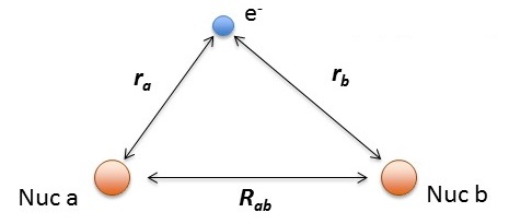
\[\hat {H} (r, R_{ab}) = -\dfrac {\hbar ^2}{2m} \nabla_a ^2 -\dfrac {\hbar ^2}{2m} \nabla_b ^2 -\dfrac {\hbar ^2}{2m} \nabla ^2 - \dfrac {e^2}{4 \pi \epsilon _0 r_a} - \dfrac {e^2}{4 \pi \epsilon _0 r_b} + \dfrac {e^2}{4 \pi \epsilon _0 R_{ab}} \label{H2+}\]

where

• \(r_a\) and \(r_a\) are the distances electron from the \(a\) and \(a\) hydrogen nuclei, respectively and
• \(R_{ab}\) is the distance between the two protons.

If we invoke the Born Oppenehimer approximation (i.e., fix the nuclear motion), we can drop the kinetic energy terms of the nuclei (notice semi-colon to represent the electronic wavefunction that depends parametrically on the geometry (\(R\)) of the system rather than a variable in the system like \(r_1\))

\[\hat {H}_{elec} (r; R_{ab}) = \underbrace{-\dfrac {\hbar ^2}{2m} \nabla ^2}_{\text{KE}} \underbrace{- \dfrac {e^2}{4 \pi \epsilon _0 r_a}}_{\text{Attract}}\underbrace{ - \dfrac {e^2}{4 \pi \epsilon _0 r_b}}_{\text{Attract}} + \underbrace{\dfrac {e^2}{4 \pi \epsilon _0 R_{ab}}}_{\text{repel/constant}} \label{H2+short}\]

This can be solved though since it is not a three-body system (only one particle is moving). What about for the hydrogen molecule?

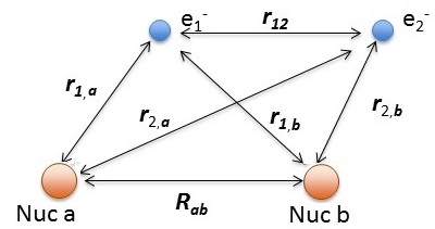
Hydrogen molecule \(H_2\) with fixed nuclei A and B, internuclear distance R. We cannot solve this analytically.

The relevant Hamiltonian (within BO approximation with fixed nuclei) is

\[\hat {H}_{elec} (r; R_{ab}) = -\dfrac {\hbar ^2}{2m} \nabla_1 ^2 -\dfrac {\hbar ^2}{2m} \nabla_2^2 - \dfrac {e^2}{4 \pi \epsilon _0 r_{1,a}} - \dfrac {e^2}{4 \pi \epsilon _0 r_{1,b}} - \dfrac {e^2}{4 \pi \epsilon _0 r_{2,a}} - \dfrac {e^2}{4 \pi \epsilon _0 r_{2,b}} + \dfrac {e^2}{4 \pi \epsilon _0 r_{12}} +\underbrace{\dfrac {e^2}{4 \pi \epsilon _0 R_{ab}}}_{\text{repel/constant}}\]

using the distances defined above.

We can analytically solve the \(H_2^+\) system (within the Born-Oppenheimer approximation), but we often do not in physical chemistry courses, since the solutions are not applicable to multi-electron diatomics. That requires an approximation like that discussed below.

The Linear Combination of Atomic Orbitals (LCAO) Approximation

First we will extend the orbital approximation from atoms to molecules, so the general multi-electron wavefunction in a molecule (at a specific configuration of nuclei, \(R\)) is

\[ | \psi (r_1, r_2, r_3 .. r_n; R) \rangle \approx | \phi_1 (r_1; R) \phi_2 (r_2; R)  \phi _3(r_3; R) ... \phi_n (r_n; R) \rangle \label{wrong}\]

where \(| \phi_n (r_n; R) \rangle\) are molecular orbitals (constructed with a specific configuration of \(R\)).

Equation \(\ref{wrong}\) is an incorrect formulation of the true multi-electron molecular wavefunction since it is an orbital approximation.

We can expand each molecular orbital into any complete basis. The one that we choose here is the basis of all atomic orbitals on all nuclei. So

\[ | \phi_i (r ; R ) \rangle = \sum _{k=1}^N \sum_{j}^{j= \infty} a_{j,k} |AO_{j,k} \rangle \label{LCAO}\]

where

• \(i\) is the index for the \(i^{th}\) molecular orbital
• \(j\) is the index for the \(j^{th}\) atomic orbitals on the \(k^{th}\) nucleus
• and \(a_{j,k}\) is the coefficient representing the amplitude (and sign) of the \(j^{th}\) atomic orbital on the \(k^{th}\) nucleus in the expansion.

To be a complete basis, this expansion must include all possible atomic orbitals, which is not numerically feasible of course. But only certain orbitals dominate the expansion (sort of like perturbation theory expansions discussed before).

This is called the Linear Combination of Atomic Orbital (LCAO) approximation for describing molecular orbitals.

The \(H_2^+\) molecular cation

The LCAO approximation is a simple method of quantum chemistry that yields a qualitative picture of the molecular orbitals in the hydrogen diatomic molecules in terms of the known atomic orbitals of the nuclei in the molecule.

\[| \phi (r) \rangle = C_A |1s_A (r)\rangle + C_B |1s_B (r) \rangle\]

We must determine the values for the coefficients, \(C_A\) and \(C_B\). We could use the linear variational method to find a value for these coefficients, but for the case of \(\ce{H2^{+}}\) evaluating these coefficients is easy by a simple use of symmetry. Since the two protons are identical, the probability that the electron is near nucleus \(A\) must equal the probability that the electron is near nucleus \(B\). These probabilities are given by \(|C_A|^2\) and \(|C_B|^2\), respectively. There are two possibilities that satisfy the condition

\[|C_A|^2 = |C_B|^2\]

namely, \(C_A = C_B = C_{+}\) and \(C_A = -C_B = C_{-}\). These two combinations produce two molecular orbitals:

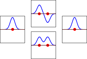
\[|\phi _+ \rangle = C_+(1s_A + 1s_B) \label{9.2.3a}\]

\[|\phi _{-} \rangle = C_{-}(1s_A - 1s_B) \label {9.2.3b}\]

These are shown below (with time dependence explicitly shown).

Electron wavefunctions for the 1s orbital of a lone hydrogen atom (left and right) and the corresponding additive molecule orbital (Equation \ref{9.2.3a}) on the bottom middle and difference molecular orbital (Equation \ref{9.2.3a}) on the top middle for the \(\ce{H2}\) molecule. The real part of the wavefunction is the blue curve, and the imaginary part is the red curve. The red dots mark the locations of the nuclei. The electron wavefunction oscillates according to the Schrödinger wave equation, and orbitals are its standing waves. (This plot is a one-dimensional slice through the three-dimensional system.). (Public Domain; Sbyrnes321).

Basis Sets

Within a linear variational method approach, the expansion of the molecular orbitals in terms of atomic orbitals in Equation \(\ref{LCAO}\) is an infinite sum. However, this is typically truncated to a finite (and feasible) sized basis set (i.e., \(j< \infty\)). The LCAO application for \(\ce{H_2^{+}}\) molecular cation uses a two-member basis set of only a 1s orbitals on each atom. However, additional atomic orbitals can be mixed in to improve the wavefunctions (marginally though).

As with typical expansions discussed in math classes, the larger the basis set (i.e., the number of terms in the expansion of Equation \ref{LCAO}), the better the resulting LCAO wavefunctions describe "reality". Although this is generally the case, there are limitations to this depending on the nature of the basis set functions and other factors (not discussed further).

Normalization and the Overlap Integral

Now we want to evaluate \(C_+\) and \(C_-\) and then calculate the energy.

a) The 1s basis functions and bonding and antibonding molecular orbitals plotted along the internuclear axis, which is defined as the z-axis, for H₂⁺. The protons are located at \(\pm\)53 pm, which corresponds to the experimental bond length. b) The electron probability density for the bonding and antibonding molecular orbitals

The constants \(C_+\) and \(C_-\) are evaluated from the normalization condition.

Example \(\PageIndex{1}\): Normalize the Bonding and Anti-bonding Molecular Orbitals for \(H_2^+\)

Normalize the \(\psi _+\) and \(\psi _{-}\) molecular orbitals formed within the LCAO approximation

Setup:

\[\int \psi ^*_{\pm} \psi _{\pm} d\tau = \left \langle \psi _{\pm} | \psi _{\pm} \right \rangle = 1 \]

\[\left \langle C_{\pm} [ 1s_A \pm 1s_B ] | C_{\pm} [ 1s_A \pm 1s_B ]\right \rangle = 1 \]

Expand:

\[|C_\pm|^2 [ \left \langle1s_A | 1s_A\right \rangle + \left \langle1s_B | 1s_B\right \rangle \pm \left \langle 1s_B | 1s_A\right \rangle \pm \left \langle1s_A | 1s_B\right \rangle] = 1 \label {9.3.3}\]

With these considerations and using the fact that \(1s\) wavefunctions are real so

\[ \left \langle 1s_A | 1s_B \right \rangle = \left \langle 1s_B | 1s_A \right \rangle = S \label {9.3.4}\]

where \(S\) is now defined as the overlap integral. Equation \(\ref{9.3.3}\) then becomes

\[|C_{\pm}|^2 (2 \pm 2S ) = 1 \label {9.3.5}\]

The solution to Equation \(\ref{9.3.5}\) is given by

\[C_{\pm} = \dfrac{1}{\sqrt{2(1 \pm S )}} \]

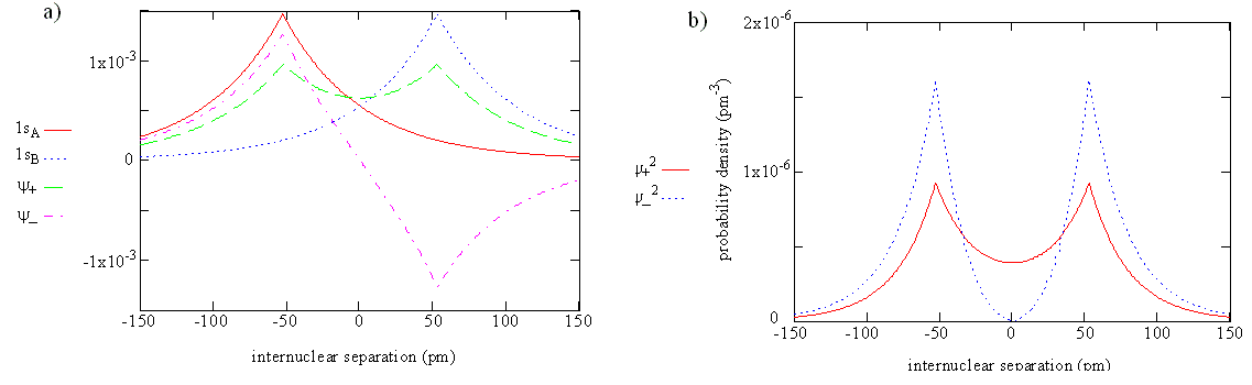
The overlap integral for two 1s atomic orbitals of hydrogen is graphically displayed below

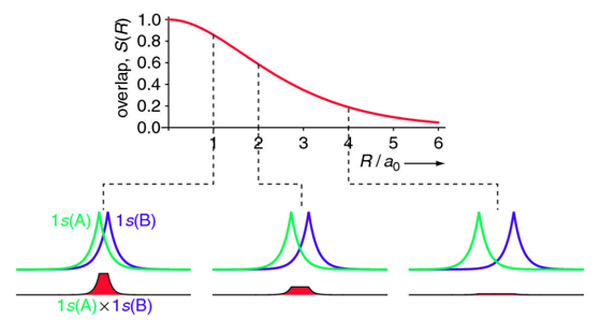
The overlap integral at different proton separations.

The overlap integral ranges from 0 to 1. If the overlap integral (\(S\)) is zero, for whatever reason, the functions are orthogonal.

The extent of overlap and thus magnitude of the overlap integral depends on \(R\). The overlap integral ranges from 0 to 1 as the separation between the protons varies from \(R = ∞\) to \(R = 0\). Clearly when the protons are infinite distance apart, there is no overlap, and when \(R = 0\) both functions are centered on one nucleus and \(\left \langle 1s_A | 1s_B \right \rangle\) becomes identical to \(\left \langle 1s_B | 1s_A \right \rangle\), which is normalized to 1, because then \(1s_A = 1s_B\).

Overlap Integral

For the overlap integral of two 1s orbitals from the hydrogen dimer discussed above is difficult to evaluate analytically and is explained here. The final answer is:

\[S(R)= \left \langle 1s_A | 1s_B \right \rangle = e^{-R/a_o} \left( 1 +\dfrac{R}{a_o} + \dfrac{R^2}{3a_o^2} \right) \nonumber\]

Example \(\PageIndex{2}\): \(S\) for the 2s-2s atomic orbitals

The overlap integral between an \(H_{2s}\) orbital and a \(H_{2s}\) orbital on nuclei separated by a distance \(R\) is:

\[S(2s,2s)=\left\{1 + \dfrac{R}{2a_0} + \dfrac{1}{12}\left(\dfrac{R}{a_0}\right)^2 + \dfrac{1}{240}\left(\dfrac{R}{a_0}\right)^4\right\} e^{-R/2a_o} \nonumber\]

Plot \(S\) as a function of \(R\). Find the ideal separation for which the overlap is a maximum.

Solution

Plot \(S\):

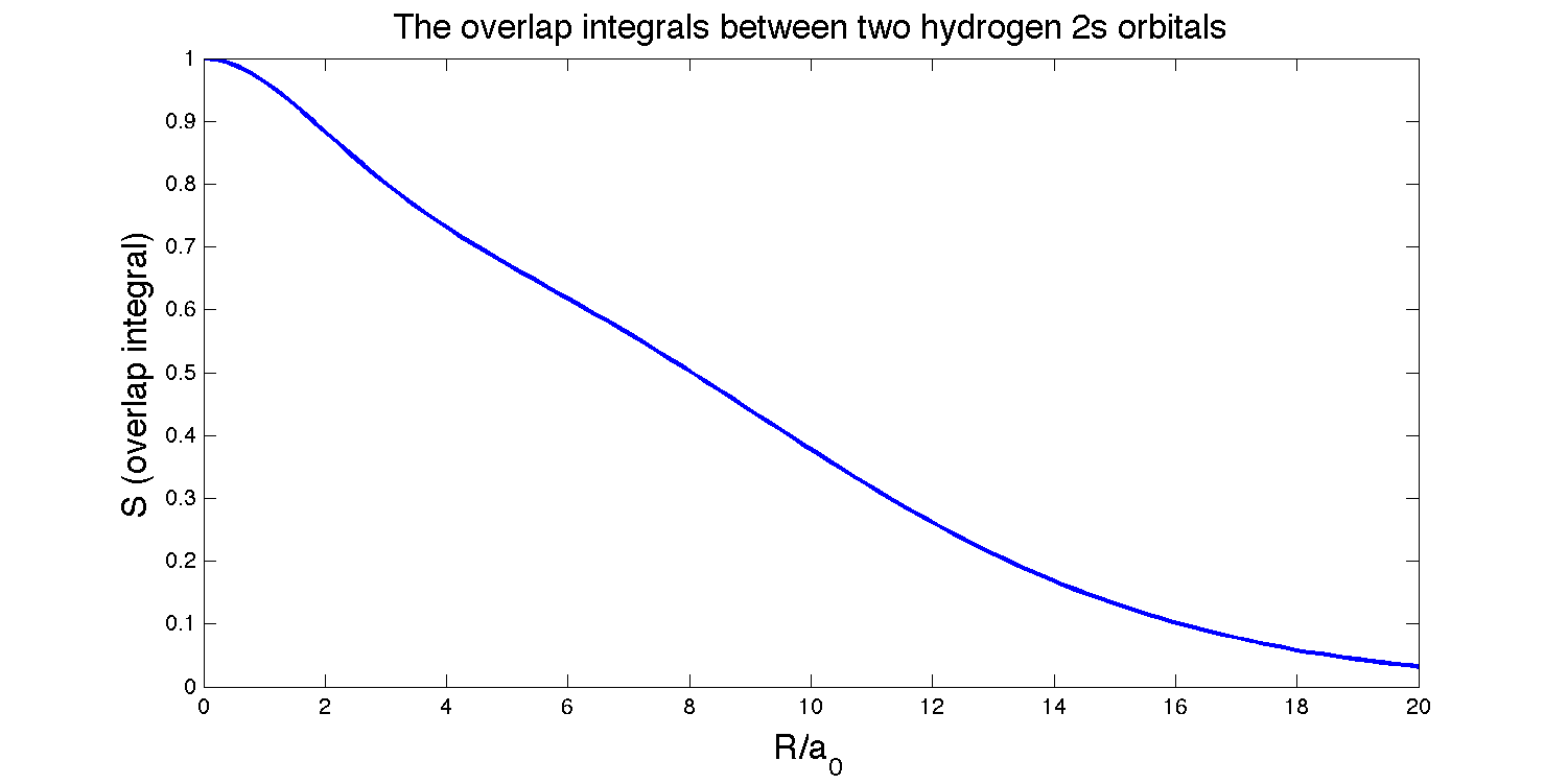
Created by Ghunbong Cheung in MATLAB

Maximize \(S\)

To find where the overlap is at its maximum, we set

\[\dfrac{dS}{dR} = 0\]

\[-\dfrac{Re^{-R/{2a_0}}(40a_0^3+20a_0^2R-8a_0R^2+R^3)}{480a_0^5} = 0\]

There are four roots for \(R\) since it is a quartic polynomial, but only one logical solution:

\[R = 0\]

This solution makes sense because these two orbitals are identical, so the maximum overlap should logical occur when the orbitals are exactly on top of each other.

Explain

Created by Ghunbong Cheung in Adobe Flash CS6

Two More Integrals

The character of \(|\psi _+ \rangle\) and \(|\psi _{-} \rangle\) molecular orbitals are reflected in the energies, which can be calculated from the expectation value of the Hamiltonian,

\[E_{\pm} = \left \langle \psi _{\pm} | \hat {H} _{elec} | \psi _{\pm} \right \rangle \label{trial energy}\]

The energy in Equation \ref{trial energy} is just the variational energy discussed previously within the linear variational method and since we are using normalized molecular orbitals, the denominator is unity and ignored.

Within the LCAO approximation that uses only 1s atomic orbital basis set expands to give

\[E_{\pm} = \dfrac {1}{2(1 \pm S)} \left[ \left \langle 1s_A |\hat {H} _{elec} | 1s_A \right \rangle + \left \langle 1s_B |\hat {H} _{elec} | 1s_B \right \rangle \pm \left \langle 1s_A |\hat {H} _{elec} | 1s_B \right \rangle \pm \left \langle 1s_B |\hat {H} _{elec} | 1s_A \right \rangle \right] \label {9.4.2a} \]

Remember: This is the variational energy for this postulated wavefunction within (linear) variational method approximation.

Notice that A and B appear equivalently with the Hamiltonian operator; this equivalence means that integrals involving 1s_A must be the same as corresponding integrals involving 1s_B, i.e.

\[ H_{AA} = H_{BB} \label {9.4.3}\]

These are called Diagonal matrix elements of the Hamiltonian in expressed in terms of the basis set we used (i.e., the 1s orbitals). If we selected a different basis, then they will change.

Since the wavefunctions are real

\[ | A \rangle = \langle A |\]

so

\[H_{AB} = H_{BA} \label {9.4.4}\]

These are called off-Diagonal matrix elements of the Hamiltonian in expressed in terms of the basis set we used (i.e., the 1s orbitals). If we selected a different basis, then they will change.

The Hamiltonian then looks like this in the this 2-element basis set

\[ \hat{H} =\begin{pmatrix}H_{AA} & H_{AB} \\H_{BA} & H_{BB}\end{pmatrix} \]

Thus Equation \(\ref{9.4.2a}\) can be written as

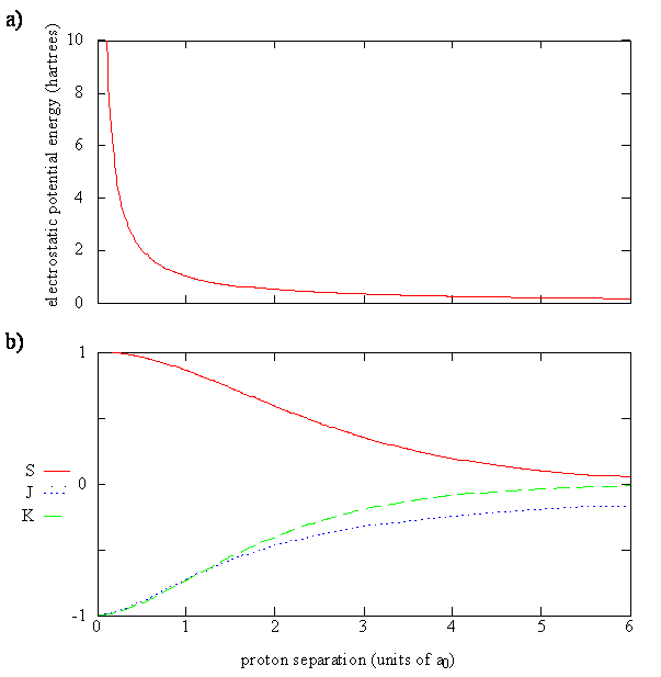
\[ \color{red} E_{\pm} (R)= \dfrac {1}{1 \pm S(R)} (H_{AA}(R) \pm H_{AB}(R)) \label {9.4.5}\]

Here the \(R\) dependence it explicitly shown. Now, let's take a closer look at the terms in this equation.

Evaluate the Diagonal Hamiltonian Matrix Elements

Now evaluate \(H_{AA}\) by inserting the Hamiltonian operator for \(H_2^+\) (Equation \ref{H2+short}) into Equation \ref{9.4.3}:

\[H_{AA} = \underset{\color{red}E_H}{ \color{black}\left \langle 1s_A \left| - \dfrac {\hbar ^2}{2m} \nabla ^2 - \dfrac {e^2}{4\pi \epsilon _0 r_A} \right| 1s_A \right \rangle } + \underset{\color{red}Columbic \; interaction}{\color{black}\dfrac {e^2}{4\pi \epsilon _0 R} \cancelto{1}{\left \langle 1s_A | 1s_A \right \rangle}} \underset{\color{red}J_{AA}}{ \color{black}- \left \langle 1s_A \left| \dfrac {e^2}{4 \pi \epsilon _0 r_B } \right| 1s_A \right \rangle } \label {9.4.6}\]

\[H_{AA} = H_{BB} = E_H + \dfrac {e^2}{4\pi \epsilon _0 R} + J_{AA} \]

• The first term is just the integral for the energy of the hydrogen atom of the 1s orbital, \(E_H\).
• The second integral is equal to 1 by normalization; the prefactor is just the Coulomb repulsion of the two protons.
• The last integral, including the minus sign, is represented by \(J\) and is called the Coulomb integral.

Physically \(J_{AA}\) is the potential energy of interaction of the electron located around proton A with proton B. It is negative because it is an attractive interaction. It is the average interaction energy of an electron described by the 1s_A function with proton B.

Coulomb Integral

The Coulomb Integral for the 1s atomic orbitals is a function of \(R\), just like \(S\) it is easiest to solve in elliptical coordinates:

\[J_{AA}(R) = - \left \langle 1s_A \left| \dfrac {e^2}{4 \pi \epsilon _0 r_B } \right| 1s_A \right \rangle = -e^{-2R/a_o} \left( 1+ \dfrac{a_0}{R} \right)\]

Off-Diagonal Hamiltonian Matrix Elements

Now consider H_AB.

\[H_{AB} = \underset{\color{red}E_H \times S}{\color{black} \left \langle 1s_A \left| - \dfrac {\hbar ^2}{2m} \nabla ^2 - \dfrac {e^2}{4\pi \epsilon _0 r_B} \right | 1s_B \right \rangle} + \underset{\color{red} S \times Columbic \; interaction}{\dfrac {e^2}{4\pi \epsilon _0 R} \cancelto{S}{\left \langle 1s_A | 1s_B \right \rangle}} - \underset{\color{red} K_{AB}}{\color{black} \left \langle 1s_A \left| \dfrac {e^2}{4 \pi \epsilon _0 r_A } \right| 1s_B \right \rangle }\label {9.4.7}\]

The first term is from the hydrogen atom Hamiltonian operating on the left (or right) to give \(E_H\) and leaving the \(S\) intergral. Equation \ref{9.4.7} then is

\[\begin{align} H_{AB} &= E_H\, S + S \dfrac {e^2}{4\pi \epsilon _0 R} + K \\[4pt] &= S \left(E_H + \dfrac {e^2}{4\pi \epsilon _0 R}\right) +K \end{align}\]

• In the first integral we have the hydrogen atom Hamiltonian and the H atom function 1s_B. The function 1s_B is an eigenfunction of the operator with eigenvalue E_H. Since E_H is a constant it factors out of the integral, which then becomes the overlap integral, \(S\). The first integral therefore reduces to E_HS.
• The second term is just the Coulombic energy of the two protons times the overlap integral.

• The third term, including the minus sign, is given the symbol \(K\) and is called the exchange integral. It is called an exchange integral because the electron is described by the 1s_A orbital on one side and by the 1s_B orbital on the other side of the operator. The electron changes or exchanges position in the molecule.

In a Coulomb integral, the electron always is in the same orbital; whereas, in an exchange integral, the electron is in one orbital on one side of the operator and in a different orbital on the other side.

Exchange Integral

For the overlap integral of two 1s orbitals from the hydrogen dimer discussed above

\[K(R)= - \left \langle 1s_A | \dfrac {e^2}{4 \pi \epsilon _0 r_A } | 1s_B \right \rangle = - e^{-R/a_o} \left( 1 + \dfrac{R}{a_0} \right)\]

Back to Energy

Now we can put these matrix element expansions (with new integrals) back into Equation \(\ref{9.4.5}\) to get the expression for the energy (of a single electron in this system)

\[E_{\pm} = E_H + \dfrac {e^2}{4\pi \epsilon _0 R} + \dfrac {J \pm K}{1 \pm S} \label {9.4.10}\]

This expression is a function of \(R\) since the three integrals outlines above are functions of \(R\) as is the Coulombic repulsion term. Equation \(\ref{9.4.10}\) tells us that the energy of the \(H_2^+\) molecule is

• the energy of a hydrogen atom plus
• the repulsive energy of two protons plus
• some additional electrostatic interactions of the electron with the protons.

These additional interactions are given by \( \dfrac {J \pm K}{1 \pm S}\). If the protons are infinitely far apart then only \(E_H\) is nonzero. To get a chemical bond and a stable H₂⁺ molecule,

1. \(\Delta E_{\pm} = E_{\pm} - E_H\) must be less than zero and
2. have a minimum, i.e. \( \dfrac {J \pm K}{1 \pm S}\) must be sufficiently negative to overcome the positive repulsive energy of the two protons \(\dfrac {e^2}{4 \pi \epsilon _0R }\) for some value of \(R\). For large R, these terms are zero, and for small R, the Coulomb repulsion of the protons rises to infinity.

(a) The electrostatic energy (in hartrees, 27.2 eV) of two protons separated by a distance R in units of the Bohr radius (52.92 pm). (b) The overlap (S), Coulomb (J), and exchange (K) integrals at different proton separations. The units for J and K are hartrees; S has no units.

Equation \(\ref{9.4.10}\) can be rewritten (by subtracting the constan \(E_H\) term) as

\[ \Delta E_{\pm} = E_{\pm} - E_H = \dfrac {e^2}{4\pi \epsilon _0 R} + \dfrac {J \pm K}{1 \pm S} \label {10.31}\]

which shows energy of \(\ce{H2^{+}}\) relative to the energy of a separated hydrogen atom (on proton and the electron) and a the other free proton. For the electron in the \(\psi_-\) orbital, the energy of the molecule, \(E_{el}(R)\), always is greater than the energy of the separated atom and proton.

Energy of the \(\ce{H2^{+}}\) bonding molecular orbital \(\Delta E_+\) and the molecular orbital \(\Delta E_-\), relative to the energy of a separated hydrogen atom and proton.

Nature wants to minimize total energy

For the electron in the \(\psi_-\) orbital, the energy of the molecule, \(E_{el}(R)\), always is greater than the energy of the separated atom and proton. That is, nature will prefer a bond to be formed to lower the energy of the system.