
5: Classical Wave Equations and Solutions (Lecture)
- Page ID
- 38870
Last lecture addressed two important aspects: The Bohr atom and the Heisenberg Uncertainty Principle. The Bohr atom was introduced because is was the first successful description of a quantum atom from basic principles (either as a particle or as a wave, both were discussed). From a particle perspective, stable orbits are predicted from the result of opposing forces (Coloumb's force vs. centripetal force). From a wave perspective, stable "standing waves" are predicted when the wavelength of the electron is an integer factor of the circumference of the the orbit (otherwise it is not a standing wave and would destructively interfere with itself and disappear). The Bohr atom predicts quantized energies that can be related to Rydberg's phenomenological spectroscopic observation (and decompose his constant \(R\) into fundamental properties of the universe and matter) via state-to-state transitions (importance for spectroscopy). This is really cool! The problem is that Bohr's theory only applied to hydrogen-like atoms (i..e, atoms or ions with a single electron). So, its quantitative utility for describing quantum chemistry is limited.
Heisenberg's Uncertainty principle is very important and is the realization that trajectories do not exist in quantum mechanics. This is commonly expressed as
\[\Delta{p}\Delta{x} \ge \dfrac{h}{4\pi} \nonumber\]
and is associated with two properties (in this case, position \(x\) and momentum \(p\). As we will show later, not all properties are dictated by Heisenberg's Uncertainly principle. We will also provide a more solid mathematical description of calculating uncertainties (with the standard deviation of a distribution).
The Heisenberg Uncertainty Principle is responsible for stopping the collapse of the hydrogen atom
According to classical mechanics, the electron would simply spiral into the nucleus and the atom would collapse. Quantum mechanics is a different story.

The total energy of a particle is the sum of kinetic and potential energies
\[E= KE + PE\]
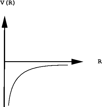
As you know, the potential energy of an electron becomes more negative as it moves toward the attractive field of the nucleus; in fact, it approaches negative infinity. However, because the total energy remains constant (a hydrogen atom, sitting peacefully by itself, will neither lose nor acquire energy), the loss in potential energy is compensated for by an increase in the electron's kinetic energy (sometimes referred to in this context as "confinement" energy) which determines its momentum and its effective velocity.
The Heisenberg principle says that either the location or the momentum of a quantum particle such as the electron can be known as precisely as desired, but as one of these quantities is specified more precisely, the value of the other becomes increasingly indeterminate.
As the electron approaches the tiny volume of space occupied by the nucleus, its potential energy dives down toward minus-infinity, and its kinetic energy (momentum and velocity) shoots up toward positive-infinity. This "battle of the infinities" cannot be won by either side, so a compromise is reached in which theory tells us that the fall in potential energy is just twice the kinetic energy, and the electron dances at an average distance that corresponds to the Bohr radius.
An electron is confined to the size of a magnesium atom with a 150 pm radius. What is the minimum uncertainty in its velocity?
- Answer
-
Start with the uncertainty principle
\[\Delta{p}\Delta{x} \ge \dfrac{\hbar}{2} \nonumber\]
can be written
\[\Delta{p} \ge \dfrac{\hbar}{2 \Delta{x}} \nonumber \]
and substituting \(\Delta p=m \Delta v \) since the mass is not uncertain.
\[\Delta{v} \ge \dfrac{\hbar}{2\; m\; \Delta{x}} \nonumber \]
the relevant parameters are
mass of electron \(m=m_e= 9.109383 \times 10^{-31}\; kg\) uncertainty in position: \(\Delta x=150 \times 10^{-12} m \)\[\Delta{v} \ge \dfrac{1.0545718 \times 10^{-34} \cancel{kg} m^{\cancel{2}} / s}{(2)\;( 9.109383 \times 10^{-31} \; \cancel{kg}) \; (150 \times 10^{-12} \; \cancel{m}) } = 3.9 \times 10^5\; m/s \nonumber\]
Waves Overview
Traveling waves, such as ocean waves or electromagnetic radiation, are waves which “move,” meaning that they have a frequency and are propagated through time and space. In contrast to traveling waves, standing waves, or stationary waves, remain in a constant position with crests and troughs in fixed intervals and specific spots of zero amplitude (node) and maximal amplitude (anti-nodes)
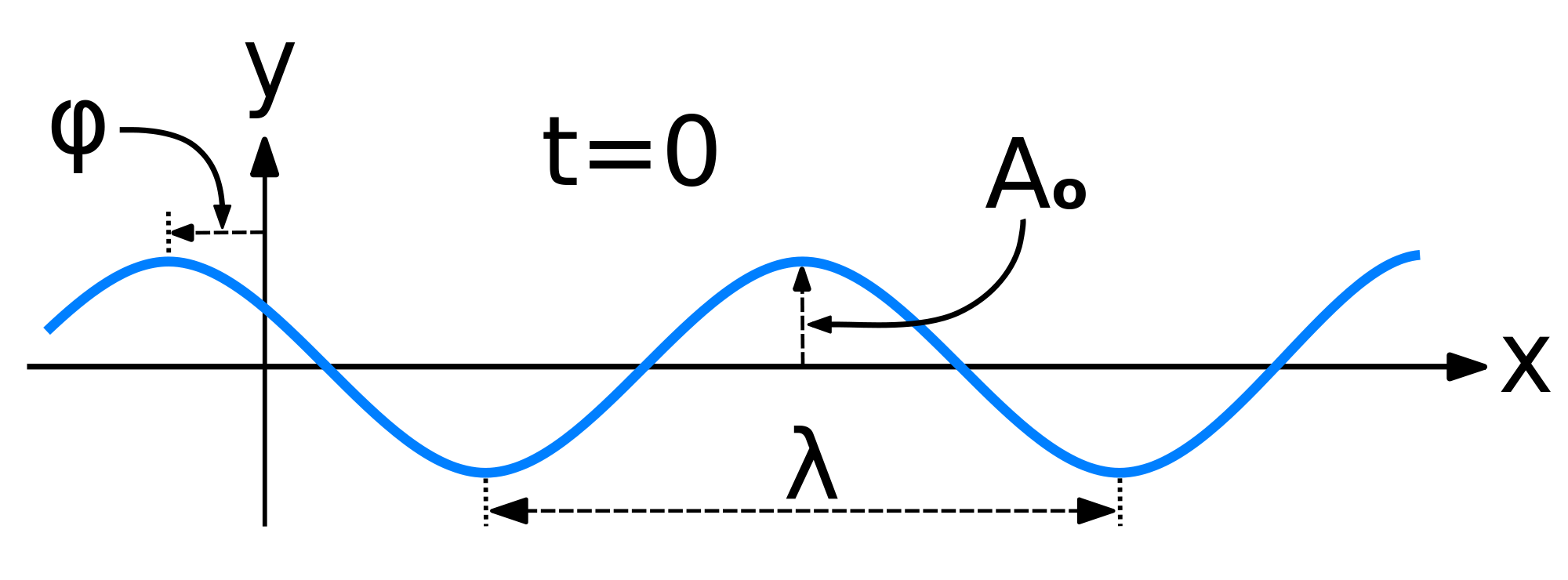
Mathematically, the most basic wave is the (spatially) one-dimensional sine wave (or harmonic wave or sinusoid) with an amplitude \(u\) described by the equation:
\[ u(x,t) = A \sin (kx - \omega t + \phi)\]
where
- \(A\) is the maximum amplitude of the wave, maximum distance from the highest point of the disturbance in the medium (the crest) to the equilibrium point during one wave cycle. In the illustration to the right, this is the maximum vertical distance between the baseline and the wave.
- \(x\) is the space coordinate
- \(t\) is the time coordinate
- \(k\) is the wavenumber
- \(\nu\) is the natural frequency
- \(\omega\) is the angular frequency (and \(\omega= 2\pi \nu\))
- \(\phi\) is the phase (with with respect to what?)
The Wave Equation
For a one dimensional wave equation with a fixed length, the function \(u(x,t)\) describes the position of a string at a specific \(x\) and \(t\) value. This leads to the classical wave equation
\[\dfrac {\partial^2 u}{\partial x^2} = \dfrac {1}{v^2} \cdot \dfrac {\partial ^2 u}{\partial t^2} \label{W1}\]
where \(v\) is the velocity of disturbance along the string. Setting boundary conditions as \(x=0\), \(u(x=0,t) = 0\) and \(x = \ell\), \(u(x=\ell , t) = 0\) allows for this partial differential equation to be solved (to see it in action in the lab see https://youtu.be/BSIw5SgUirg?t=17). Assuming the variables \(x\) and \(t\) are independent of each other makes this differential equation easier to solve, as you can use the Separation of Variables technique.
The separation of variables is common method for solving ordinary and partial differential equations, in which algebra allows one to rewrite an equation so that each of two variables occurs on a different side of the equation.
In this case, separation of variables "anzatz" says that
\[u(x,t) = X(x)T(t) \label{ansatz}\]
"An ansatz is the establishment of the starting equation(s), the theorem(s), or the value(s) describing a mathematical or physical problem or solution. It can take into consideration boundary conditions. After an ansatz has been established (constituting nothing more than an assumption), the equations are solved for the general function of interest (constituting a confirmation of the assumption)." - Wikipedia

Substituting Equation \ref{ansatz} into Equation \(\ref{W1}\) gives
\[T(t) \cdot \dfrac {\partial ^2 X(x)}{\partial x^2} = \dfrac {X(x)}{v^2} \cdot \dfrac {\partial ^2 T(t)}{\partial t^2}\]
which simplifies to
\[\dfrac {1}{X(x)} \cdot \dfrac {\partial ^2 X(x)}{\partial x^2} = \dfrac {1}{T(t) v^2} \cdot \dfrac {\partial ^2 T(t)}{\partial t^2} = K\]
where \(K\) is called the "separation constant". By setting each side equal to \(K\), two 2nd order homogeneous ordinary differential equations are made.
\[\dfrac {d^2 X(x)}{d x^2} - KX(x) = 0 \label{spatial}\]
and
\[\dfrac {d^2 T(t)}{d t^2} - K v^2 T(t) = 0 \label{time}\]
We are particular interest in this example with specific boundary conditions (the wave has zero amplitude at the ends).
\[u(x=0,t)=0\]
\[u(x=L,t)=0\]
This should sound familiar since we did it for the Bohr hydrogen atom (but with the line curved in on itself)
Solving the Spatial Part
Solving the spatial part (Equation \ref{spatial}):
\[\dfrac {\partial ^2 X(x)}{\partial x^2} - KX(x) = 0 \label{spatial1}\]
Equation \ref{spatial} is a constant coefficient second order linear ordinary differential equation (ODE), which had general solution of
\[X(x) = A\cdot \cos \left(a x \right) + B\cdot \sin \left(b x\right) \label{gen1}\]
However, these general solutions can be narrowed down by addressing the boundary conditions. Because of the separation of variables above, \(X(x)\) has specific boundary conditions (that differ from \(T(t)\)):
- \(X(x=0) = 0\)
- \(X(x=\ell) = 0\).
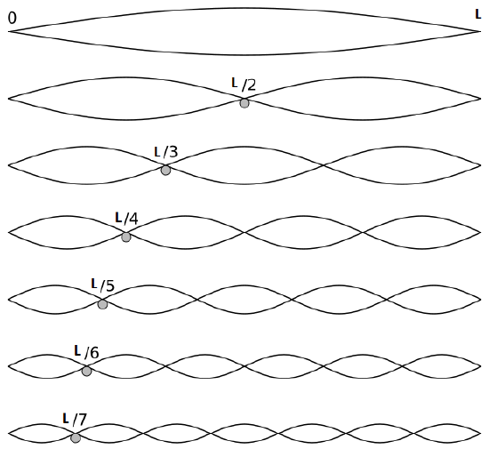
So there is no way that any cosine function can satisfy the boundary condition (try it if you do not believe me) - hence, \(A=0\). Moreover, only functions with wavelengths that are integer factors of half the length (\(i.e., n\ell/2\)) will satisfy the boundary conditions. So Equation \ref{gen1} simplifies to
\[X(x) = B\cdot \sin \left(\dfrac {n\pi x}{\ell}\right)\]
where \(\ell\) is the length of the string, \(n = 1, 2, 3, ... \infty\), and \(B\) is a constant. By substituting \(X(x)\) into the partial differential equation for the temporal part (Equation \ref{spatial1}), the separation constant is easily obtained to be
\[K = -\left(\dfrac {n\pi}{\ell}\right)^2 \label{Kequation}\]
Solving the Temporal Part
Plugging the value for \(K\) from Equation \ref{Kequation} into the temporal component (Equation \ref{time}) and then solving to give the general solution (for the temporal behavior of the wave equation):
\[T(t) = D\cos \left(\dfrac {n\pi\nu}{\ell} t\right) + E\sin \left(\dfrac {n\pi\nu}{\ell} t\right) \label{gentime}\]
where \(D\) and \(E\) are constants and \(n\) is an integer (\(\gt 1\)), which is shared between the spatial and temporal solutions.
Unfortunately, we do not have the boundary conditions like with the spatial solution to simplify the expression of the general temporal solutions in Equation \ref{gentime}. However, these solutions can be simplified with basic trigonometry identities to
\[T_n (t) = A_n \cos \left(\dfrac {n\pi\nu}{\ell} t +\phi_n\right) \label{timetime}\]
where \(A_n\) is the maximum displacement of the string (as a function of time), commonly known as amplitude, and \(\phi_n\) is the phase and \(n\) is the number from required to establish the boundary conditions.
The evolution of Equation \ref{gentime} into Equation \ref{timetime} originates from the sum and difference trigonometric identites. This requires reformulating the \(D\) and \(E\) coefficients in Equation \ref{gentime} in terms of two new constants \(A\) and \(\phi\)
\[D= A \cos(\phi) \nonumber\]
and
\[E= A \sin(\phi) \nonumber\]
Equation \ref{gentime} then looks like
\[T(t) = A \cos (\phi) \cos \left(\dfrac {n\pi\nu}{\ell} t\right) + A \sin (\phi) \sin \left(\dfrac {n\pi\nu}{\ell} t\right) \label{gentime3}\]
we use the sum trigonometric identity:
\[\cos (A+B) \equiv \cos\;A ~ \cos\;B ~-~ \sin\;A ~ \sin\;B\label{eqn:sumcos}\]
to rewrite rewrite Equation \ref{gentime3} into Equation \ref{timetime}.
The Total Package: The Spatio-temporal solutions are Standing Waves
Remembering base the Anzatz in this procedure, \(u_n (x,t) = X(x) T(t)\), and substituting in our determined \(X\) and \(T\) functions gives
\[u_n = A_n \cos(\omega_n t +\phi_n) \sin \left(\dfrac {n\pi x}{\ell}\right)\]
The first six wave solutions \(u(x,t;n)\) are standing waves with frequencies based on the number of nodes (0, 1, 2, 3,...) they exhibit (more discussed in the following Section).
Since the acceleration of the wave amplitude is proportional to \(\dfrac{\partial^2}{\partial x^2}\), the greater curvature in the material produces a greater acceleration, i.e., greater changing velocity of the wave and greater frequency of oscillation. As discussed later, the higher frequency waves (i..e, more nodes) are higher energy solutions; this as expected from the experiments discussed in Chapter 1 including Plank's equation \(E=h\nu\).
The higher frequency waves are higher energy solutions.
Superposition
Since the wave equation is a linear homogeneous differential equation, the total solution can be expressed as a sum of all possible solutions.
\[\begin{align} u(x,t) &= \sum_{n=1}^{\infty} a_n u_n(x,t) \\ &= \sum_{n=1}^{\infty} \left( G_n \cos (\omega_n t) + H_n \sin (\omega_n t) \right) \sin \left(\dfrac{n\pi x}{\ell}\right) \end{align}\]
The waveform at a given time is a function of the sources (i.e., external forces, if any, that create or affect the wave) and initial conditions of the system. In many cases (for example, in the classic wave equation), the equation describing the wave is linear. When this is true, the superposition principle can be applied. That means that the net amplitude caused by two or more waves traversing the same space is the sum of the amplitudes which would have been produced by the individual waves separately. For example, two waves traveling towards each other will pass right through each other without any distortion on the other side.
The \(u_n(x,t)\) solution is called a normal mode. This sort of expansion is ubiquitous in quantum mechanics.
This java applet is a simulation that demonstrates standing waves on a vibrating string. www.falstad.com/loadedstring/
Everything above is a classical picture of wave, not specifically quantum, although they all apply. We will introduce quantum tomorrow and the waves will be wavefunctions. Since the Schrödinger equation (that is the quantum wave equation) is linear, the behavior of the original wave function can be computed through the superposition principle.
Expansions are important for many aspects of quantum mechanics.