
10.2: Gas Laws
- Page ID
- 52148

Gas Phase Chemistry
Gasses are compressible fluids which form homogenous solutions. An ideal gas is a gas where there are no attractive (or repulsive) forces between the particles and their kinetic energy (the energy of motion) is linearly proportional to the absolute temperature (K). This relationship is expressed by the Ideal Gas Law as presented in the last section.
\[PV=nRT \\variables = P,V,n,T \\constant = R=0.082057\left (\frac{L\cdot atm}{mol\cdot K} \right)\]
The value of the Ideal Gas constant R depends on the units. The bottom left unit of table \(\PageIndex{1}\) (R=8.314 \(\left ( \frac{J}{mol\cdot K} \right )\)) is of special significance and will be used extensively in the second semester of this class (when you will need to memorize that value), as it relates the energy (Joules) of a gas to the absolute Temperature (K) and number of gas particles in the gas (n). In this class you only need to memorize the first value to four significant digits, (R=0.08206 \(\left (\frac{L\cdot atm}{mol\cdot K} \right)\). And hopefully you have realized by now that all these constants can be converted to SI base units (bottom right value of table, which is expressed in units of kg, m, mol and second).
| R=0.082057 \(\left (\frac{L\cdot atm}{mol\cdot K} \right) \) | R=62.36367 \(\left ( \frac{L\cdot torr}{mol\cdot K} \right )\) |
| R=8.3144598 \(\left ( \frac{J}{mol\cdot K} \right )\) | R=8.3144598 \(\left ( \frac{kg(m^{2})}{(s^{2})mol\cdot K} \right )\) |
In the next section we will develop the empirical gas laws. What is important is that you be able to derive these from the ideal gas law.
Empirical Gas Laws
Empirical data is experimental data, and an experiment typically involves two variables, the independent variable, which we change, and the dependent variable, whose value changes as the independent variable is changed. We generically define these variables as (X,Y) where X is the independent and Y is the dependent variable, and then set up an equation where Y is a function of X, or Y =fct(X). A common function is the linear function as expressed in fig. 10.2.1
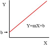
Figure \(\PageIndex{1}\): Linear function where the value of Y (dependent variable) depends on the value of X (independent variable).
If we take a closer look at the ideal gas law, we see there are four variables, (P, T, V and n) and 1 constant (R). To make a plot of n variables you need n-dimensions. So two variables gives a line, three gives a surface (x,y,x axes), and there is no way we can draw 4 variables. What the early scientists could do is hold 2 of the 4 variables constant, and make 2D plots, and the empirical gas laws are the plots that result in linear equations. These were historically determined, and then later the Ideal gas law was developed. But we can use each of the empirical gas laws as a special case of the ideal gas law, defined by which variables are constant, and which are measured. So the idea is simple, you hold two variables constant, change the third (independent variable) and observe how the fourth adjusts (dependent variable).
The Ideal Gas Law can be written as \[\frac{PV}{nT}=R\]
Each of the Empirical Gas laws is an expression of the above equation where two of the four variables are held constant, and thus each of the empirical gas constants is related to the Ideal Gas constant through the values of the variables that were held constant.
Boyle's Law (constant n,T)
PV=Constant
This describes the relationship between the pressure and volume of a gas with a constant number of particles at constant temperature.
From the Ideal Gas Law we would predict:
\[PV=nRT\Rightarrow V=\left ( nRT \right )\frac{1}{P}\]
since n, R and T are all constants, we have
\[PV=k\]
\[PV=k~~where,k=\left ( nRT \right )\]
Note, there are two possible graphs that come out of this relationship,
- P vs. 1/V
- V vs. 1/P
These graphs of of the form Y=function of X, where Y is the dependent variable and x is the independent variable. That is, if you change X, how does Y change? So if I have a sealed cylinder and I double the volume the pressure will change and so one would plot pressure as a function of volume. But if you had a frictionless piston in a cylinder and then changed the pressure in the cylinder, the piston would move until a new equilibrium was achieved, and we would say the volume is a function of pressure.
Part (a) of Figure 10.2.2 shows that P and V are not linear, but as predicted above and shown in part (b), V is linear to the reciprocal of P.
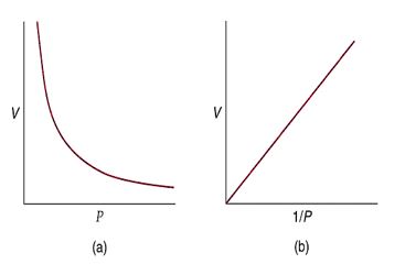
Figure \(\PageIndex{2}\): Plot (a) shows a non linear relationship of V as a function of P, while (b) shows V and P are inversely related.
What the data says is that as P goes down, 1/P goes up, and V goes up proportional to 1/P.
Note
This might be easier to understand if we switched the axes and look at how the pressure is dependent on the volume.
\[P=k'\frac{1}{V} \; \text{where, k=}\frac{1}{k'}\]
The pressure is the force per unit area, and the pressure is due to the collision of gas particles against the surface of the container. The greater the collision frequency of particles with the wall, the greater the pressure. If you have a gas in a rigid container and reduce its volume, 1/V goes up, and the pressure goes up because there is a shorter path distance between the walls (increasing the collision frequency).
We will revisit this after we cover the Kinetic Molecular Theory of gases, where you will find a better explanation (section 10.5.4).
Gay-Lussac's Law (constant n,V)
\(\frac{P}{T}=Constant\)
This describes the relationship between the pressure and temperature of a gas with a constant number of particles at constant temperature. From the Ideal Gas Law we would predict:
PV=nRT \(\Rightarrow P=\left ( \frac{nR}{V} \right )T\)
since n,V & R are constants
P=kT where, k=\(\left ( \frac{nR}{V} \right )\)
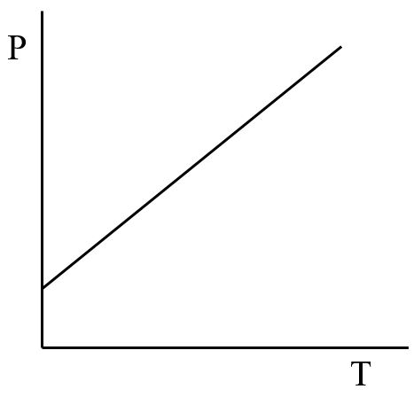
This describes a rigid closed container containing a fixed number of gas particles. As the temperature goes up the particles move faster, hit the wall more frequently at higher velocities and so the pressure goes up (remember P=\(\frac{F}{A}\). As the temperature rises the pressure continues to rise and at some point the material of the rigid container will rupture and an explosion will occur as the gas escapes.
Likewise, as the temperature goes down the molecules slow down, hit the wall less frequently at lower velocities and so the pressure drops. Note, there is a lower limit to this equations, which is defined as the boiling point, and at temperatures below that Temperature the particle condenses out as a liquid (it is no longer a gas), and the Ideal gas law does not describe the system.
Charles's Law (Constant n,P)
This describes the relationship between the volume and the temperature of a gas with a constant number of particles at constant pressure. This relationship is demonstrated in the following YouTube where a balloon full of air is dropped into liquid nitrogen, and then returned to room temperature.
Mathematically, Charles's Law can be derived from the ideal gas equation at constant pressure and number of particles and would be modeled by an ideal balloon (closed system) that had no resistance to expansion or contraction (constant pressure).
\[PV=nRT\Rightarrow V=\left ( \frac{nR}{P} \right )T \Rightarrow V=kT \; where,k=\left ( \frac{nR}{P} \right )\; or \;T=k'V \; where, k=\frac{1}{k'}\]
Note, just as for Gay-Lussac's Law there is a lower limit for the temperature, being the "boiling point", at which temperature the gas converts to a liquid and no longer follows the gas laws. Figure \(\PageIndex{4}\) shows experimental (empirical) data for the volume of a gas as a function of temperature.
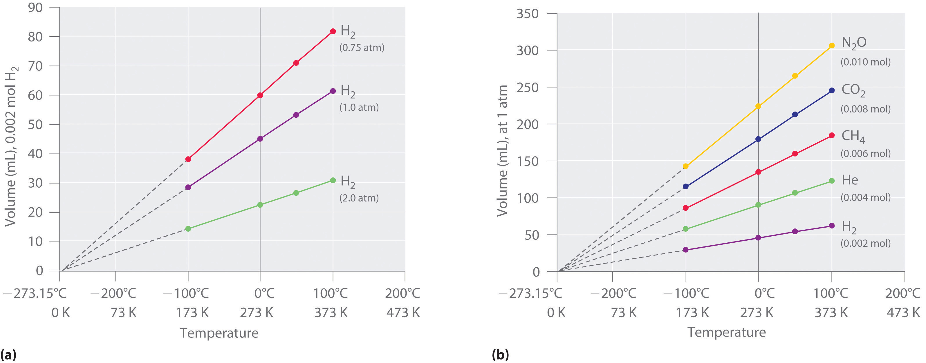
Figure \(\PageIndex{4}\): The Relationship between Volume and Temperature. (a) In these plots of volume versus temperature for equal-sized samples of H2 at three different pressures, the solid lines show the experimentally measured data down to −100°C, and the broken lines show the extrapolation of the data to V = 0. The temperature scale is given in both degrees Celsius and kelvins. Although the slopes of the lines decrease with increasing pressure, all of the lines extrapolate to the same temperature at V = 0 (−273.15°C = 0 K). (b) In these plots of volume versus temperature for different amounts of selected gases at 1 atm pressure, all the plots extrapolate to a value of V = 0 at −273.15°C, regardless of the identity or the amount of the gas (CC BY-SA-NC; anonymous by request).
The significance of the invariant T intercept in plots of V versus T was recognized in 1848 by the British physicist William Thomson (1824–1907), later named Lord Kelvin. He postulated that −273.15°C was the lowest possible temperature that could theoretically be achieved, for which he coined the term absolute zero (0 K).
Avogadro's Law (Constant P,T)
This describes the relationship between the volume and the number of particles in a gas at constant pressure and temperature. We can derive Avogadro's Law from the ideal gas law using these constants:
\[PV=nRT, \; \; \; \; \; \; \small{\text{at constant P,T}} \\ V=\left ( \frac{RT}{P} \right )n, \; \; \; \; \; \; \; \; \small{where \; k=\left ( \frac{RT}{P} \right )} \\ \Large{V=kn}\]

An important facet of Avodadro's Law is that this relationship does not depend on the identity of the molecule (we will learn later that there are deviations), but the value of the constant does depend on the value of P and T held constant
Historically, around 1811 Avogadro postulated his hypothesis, which was that equal volumes of gasses contain equal numbers of particles, and Avogadro's Law derives from that relationship. It is common to use STP (standard temperature and pressure) as the value for the constants (T and P) in Avagadro's Law
STP (Standard Temperature and Pressure)
STP is the standard temperature and pressure that many gas values are tabulated at. You may notice different values in different textbooks because in 1982 the definiton of the standard pressure changed from 1 atm to 1 bar.
- Until 1982, STP was defined as a T= 0 °C and P = 1 atm (101.325 kPa).
- Since 1982, STP is defined as a T= 0 °C and P = 1 bar (100kPa)
Molar Volume at STP
Avogadro's hypothesis states that the volume of a mole should be the same for any substance, and as can be seen from Table \(\PageIndex{1}\).
| Substance | Formula | Molar Volume/liter mol–1 |
|---|---|---|
| Hydrogen | H2(g) | 22.43 |
| Neon | Ne(g) | 22.44 |
| Oxygen | O2(g) | 22.39 |
| Nitrogen | N2(g) | 22.40 |
| Carbon dioxide | CO2(g) | 22.26 |
| Ammonia | NH3(g) | 22.09 |
The data in Table \(\PageIndex{1}\), then, indicate that for a variety of gases, 6.022 × 10²³ molecules occupy almost exactly the same volume (the molar volume) if the temperature and pressure are held constant, and the molar volume for an ideal gas is 22.4 l/mol. So if you can measure the volume of a gas at STP, you can calculate the number of moles.
Ideal Gas Law Calculations
There are three basic types of calculations involving the ideal gas law
- PV=nRT calculations.
- Calculations involving Density and formula weights.
- Two State Problems
PV=nRT
These are simple algebraic problems where you are given 3 of the 4 variables. The trick is to keep your units in your equations and be sure the units of the answer make sense. If you think about it, the numerical value of R depends on the units of R (see table 10.2.1), and your variables must have the units of R or they will not cancel. This is especially important for temperature, which must be in units of Kelvin.
Exercise \(\PageIndex{1}\)
The following problems represent various solutions to the ideal gas equation
- A sample of gaseous Cl2 has a volume of 12.4 L at 500.0 K and 0.521 atm. How many moles are present?
- What is the mass of chlorine gas in a 12.4L container at 500.0K and 0.521 atm?
- What volume is occupied by 1.06 mol of CO2 gas at 299 K and a pressure of 0.89 atm?
- What is the temperature of 1.41 mol of methane gas in a 5.0 L container at 1.00 atm?
- What is the pressure exerted by a 1.75 mol sample of water at 7.0L and 20oC?
- Answer a
-
\[n=\frac{PV}{RT}=\frac{0.521atm\left ( 12.4L \right )}{0.08206\frac{L\cdot atm}{mol\cdot K}\left ( 500K \right )}=0.157mol \nonumber \]
- Answer b
-
\[n=\frac{PV}{RT}=\frac{0.521atm\left ( 12.4L \right )}{0.08206\frac{L\cdot atm}{mol\cdot K}\left ( 500K \right )}=0.157mol \nonumber \]
\[0.157mol~Cl_{2}\left ( \frac{70.90g~Cl_{2}}{mol} \right )=11.1g\]
- Answer c
-
\[V=\frac{nRT}{P}=\frac{1.06mol\left ( 0.08206\frac{L\cdot atm}{mol\cdot K} \right )299K}{0.89atm}=29L \nonumber \]
- Answer d
-
\[T=\frac{PV}{nR}=\frac{1.00atm\left ( 5.0L \right )}{1.41mol\left ( 0.08206\frac{L\cdot atm}{mol\cdot K} \right )}=43K \nonumber \]
- Answer e
-
\[P=\frac{nRT}{V}=\frac{1.75mol\left ( 0.08206\frac{L\cdot atm}{mol\cdot K} \right )293.15K}{7.0L}=6.0atm \nonumber \]
Density and formula weight.
The formula weight of a compound can be expressed in terms of the number of moles, where\[\ fw(\frac{g}{mol})=\frac{m(g)}{n(mol)} \]
solving for n:
\[n=\frac{m}{fw}\]
Substituting for n in the ideal gas law (PV=nRT) gives:
\[ PV=\left (\frac{m}{fw} \right )RT\]
This allows us to solve for both density and the formula weight
1. Density
Rearranging eq. 10.2.9 to \(d=\frac{m}{V}\) gives
\[d=\frac{m}{V}=\frac{P(fw)}{RT}\]
2. Formula Weight
Solving Equation 10.2.9 directly for formula weight gives
\[fw=\frac{mRT}{PV}=\left ( \frac{m}{V} \right )\frac{RT}{P}=\frac{dRT}{P}\]
note how the above eq. can be expressed in terms of density, or mass and volume.
Example \(\PageIndex{1}\): Calculating the formula weight from density, pressure and temperature.
What is the formula weight of an unknown gas if it has a density of 4.08g/l at 88 °C and 1.4 atm?
Solution
NOTE: There are many ways you can solve this problem, and in video we note that we are looking for the formula weight, and so we start with an equation that has the formula weight, and solve it for the formula weight by identifying what variables we do not have, and substituting for them.
If you know the identity of a gas, you know its formula weight. The following problem calculates the density of a gas if we know what it is. In solving this it is good to reflect on the fact that a gas is compressible, that is, it expands or contracts to a change in volume. So you can not use the simple \(d=\frac{m}{v}\) that you could use for an incompressible substance like a liquid or a solid.
Example \(\PageIndex{2}\): Calculating the density of a known gas at a given temperature and pressure
What is the density of sulfur dioxide gas at 88 deg C and 1.4 atm?
Solution
Note, since we know what the gas is, we know its formula weight. Since we are solving for density, we start with the density equation.
Example \(\PageIndex{3}\): Determining the Molar Mass of a Volatile Liquid
The approximate molar mass of a volatile liquid can be determined by:
- Heating a sample of the liquid in a flask with a tiny hole at the top, which converts the liquid into gas that may escape through the hole
- Removing the flask from heat at the instant when the last bit of liquid becomes gas, at which time the flask will be filled with only gaseous sample at ambient pressure
- Sealing the flask and permitting the gaseous sample to condense to liquid, and then weighing the flask to determine the sample’s mass (Figure \(\PageIndex{1}\))
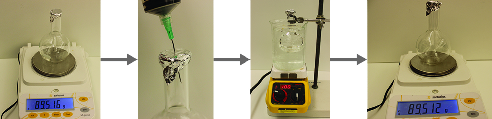
Using this procedure, a sample of chloroform gas weighing 0.494 g is collected in a flask with a volume of 129 cm3 at 99.6 °C when the atmospheric pressure is 742.1 mm Hg. What is the approximate molar mass of chloroform?
Solution
Since
\[fw=\dfrac{m}{n} \]
and
\[n=\dfrac{PV}{RT} \]
substituting and rearranging gives
\[fw=\dfrac{mRT }{PV}\]
then
\[fw=\dfrac{mRT}{PV}=\mathrm{\dfrac{(0.494\: g)×0.08206\: L⋅atm/mol\: K×372.8\: K}{0.976\: atm×0.129\: L}=120\:g/mol} \]
Two State Approach
If you have a gaseous system and then perturb it by changing one of more variables the other variables adjust to that change. The two state approach is a quick way to solve these problems. The idea is simple, you have a relationship PV=nRT, so at one state, P1V1 =n1RT1 and P2V2=n2RT2 , so we can set up the equivalence:
\[ \frac{P_{1}V_{1}}{P_{2}V_{2}}=\frac{n_{1}RT_{1}}{n_{2}RT_{2}}=\frac{n_{1}T_{1}}{n_{2}T_{2}}\]
so
\[\frac{P_{1}V_{1}}{P_{2}V_{2}}= \frac{n_{1}T_{1}}{n_{2}T_{2}} \]
(note: the constant (R) cancels out)
Warning: T must be in Kelvin, as the equation PV=nRT requires T to be in Kelvin, and even though R cancels in the two state approach, T still needs to be in Kelvin.
When solving these problems it is wise to make a table and write down what you are given. If something is held constant, it cancels out of the equation.
| State 1 | State 2 |
|---|---|
| T1= | T2= |
| P1= | P2= |
| V1= | V2= |
| n1= | n2= |
Example \(\PageIndex{3}\)
What is the volume of a perfectly elastic balloon if it rises to an altitude where the pressure drops to 0.100 atm and the temperature drops to 173 K if it had a volume of 5.00 liters at sea level where the pressure was 1.00 atm and the temperature was 273K?
Solution
(a) Set up two state equation and solve for V1 or V2 (which either is easier, as we have not assigned the data to the states
\[\frac{P_{1}V_{1}}{P_{2}V_{2}}= \frac{n_{1}T_{1}}{n_{2}T_{2}} \\ \; \\ becomes \\ \; \\ V_1=V_2\left ( \frac{n_1}{n_2} \right )\left ( \frac{T_1}{T_2} \right )\left ( \frac{P_2}{P_1} \right )\]
(b) Fill our the data table so we properly identify the data with the state.
TIP, Since we want the volume in the upper atmosphere we will call that state 1, but we could have called sea level state one, in which case we would solve for V2.
| State 1 | State 2 |
|---|---|
| T1= 173K | T2= 273K |
| P1= 0.100 atm | P2= 1.00 atm |
| V1= ? | V2= 5.00 L |
| n1= | n2= |
NOTE: This is a closed system and no gas entered or escaped from the balloon and so n1=n2 and they cancel.
\[V_1=5.00L\cancel{ \left ( \frac{n_1}{n_2} \right )} \underbrace{ \left ( \frac{173 K}{273 K} \right )}_{\color{red}{T \; must \; be \\ in \; Kelvin}} \left ( \frac{1 atm}{0.100 atm} \right )\]
The solution to this problem is demonstrated in video \(\PageIndex{4}\).
Note
Many textbooks cover the "combined gas law":
\[\frac{P_1V_2}{T_1}=\frac{P_2V_2}{T_2}\]
On closer inspection the combined gas law is applying the two-state approach to the ideal gas law where n, the number of molecules is constant, and that was the case we just solved (example 10.3.2). The advantage of the two state approach is that it not only allows us to handle changes in the number of particles, but it is a technique that can be applied to many equations, not just the ideal gas equation.
If you have a relationship y=mx, you can always say that \(\frac{y_1}{y_2}=\frac{x_2}{x_2}\), and during the second semester this technique will be applied to power functions (Y=AXm) and exponential functions Y=Aexm. It is worth mastering the two state approach now.
Exercise \(\PageIndex{2}\)
Solve the following problems using the two state approach.
- What pressure would 6.1 moles of a gas in a rigid container have at 20.0 oC have if it had a pressure of 0.45 atm at -45.0 oC?
- A pressure tank containing chlorine gas at a pressure of 2.00 atm and a temperature of 40oC is set with a pressure relief valve set to open at a pressure of 10.0 atm. At what temperature will the relief valve open?
- A gas is in a sealed cylinder at 25oC with a piston which can expand or contract to change the volume. The initial volume and pressure are 75.0 L and 980.0 torr. A force is applied to the piston and the volume adjusts to a final pressure and temperature of 5.00 atm at 188oC. What is the final volume?
- Answer a
-
\[P_{1}=P_{2}\frac{T_{1}}{T_{2}}=\left ( 0.45atm \right )\left ( \frac{293.15K}{228.15K} \right )=0.58atm\]
- Answer b
-
\[T_{2}=T_{1}\frac{P_{2}}{P_{1}}= \left ( 313.15K \right )\left ( \frac{10.0atm}{2.00atm} \right )=1570K\]
- Answer c
-
\[V_{2}=V_{1}\left ( \frac{P_{1}}{P_{2}} \right )\left ( \frac{T_{2}}{T_{1}} \right )=75.0L\left ( \frac{980torr\left ( \frac{1atm}{760torr} \right )}{5.00atm} \right )\left ( \frac{461.15K}{298K} \right )=29.9L\]
Contributors and Attributions
- Bob Belford (UALR) and November Palmer (UALR)
- Adoptions from Openstax