1B.5: Graphs and Graphing

Last updated
Save as PDF

Page ID: 50465

\( \newcommand{\vecs}[1]{\overset { \scriptstyle \rightharpoonup} {\mathbf{#1}} } \) \( \newcommand{\vecd}[1]{\overset{-\!-\!\rightharpoonup}{\vphantom{a}\smash {#1}}} \)\(\newcommand{\id}{\mathrm{id}}\) \( \newcommand{\Span}{\mathrm{span}}\) \( \newcommand{\kernel}{\mathrm{null}\,}\) \( \newcommand{\range}{\mathrm{range}\,}\) \( \newcommand{\RealPart}{\mathrm{Re}}\) \( \newcommand{\ImaginaryPart}{\mathrm{Im}}\) \( \newcommand{\Argument}{\mathrm{Arg}}\) \( \newcommand{\norm}[1]{\| #1 \|}\) \( \newcommand{\inner}[2]{\langle #1, #2 \rangle}\) \( \newcommand{\Span}{\mathrm{span}}\) \(\newcommand{\id}{\mathrm{id}}\) \( \newcommand{\Span}{\mathrm{span}}\) \( \newcommand{\kernel}{\mathrm{null}\,}\) \( \newcommand{\range}{\mathrm{range}\,}\) \( \newcommand{\RealPart}{\mathrm{Re}}\) \( \newcommand{\ImaginaryPart}{\mathrm{Im}}\) \( \newcommand{\Argument}{\mathrm{Arg}}\) \( \newcommand{\norm}[1]{\| #1 \|}\) \( \newcommand{\inner}[2]{\langle #1, #2 \rangle}\) \( \newcommand{\Span}{\mathrm{span}}\)\(\newcommand{\AA}{\unicode[.8,0]{x212B}}\)

Learning Objectives

Define independent and dependent values
Recognize the different types of functions
Generate an algebraic expression for data from a graph
Recognize units of temperature and how they were derived graphically
Convert between different scales of temperature

Introduction

A graph can be used to show the relationship between two related values, the dependent and the independent variables.

Dependent Variable: A measurable variable whose value depends on the independent variable. Often represented by the algebraic symbol y.
Independent Variable: A measurable variable of which when changed, the value of the dependent variable changes. Often represented by the algebraic symbol x.

\[y=\text{function of x} \\ or \\ y=f(x)\]

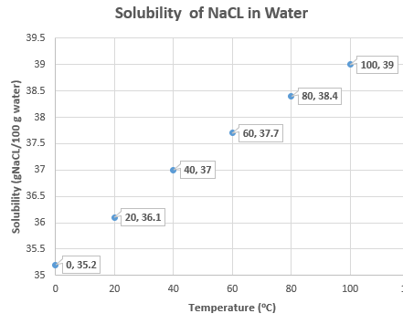
Such a relationship would be the maximum amount of table salt (sodium chloride) you can dissolve in water as a function of temperature, which is represented by the data in table 1B.5.1. This represents a saturated solution, and what you notice is that if you raise the temperature of the water more table salt can dissolve. That is, if you have 26.1 g salt at 20.0 ^oC dissolved in 100 grams of water (which is the maximum amount that can dissolve in 100 grams of water), and add another 2 grams, it just falls to the bottom of the solution and the temperature does not change. If you then raise the temperature the solid at the bottom starts to dissolve and somewhere around 70 degrees all the salt dissolves. So the solubility is the dependent variable, and its value depends on the temperature, the independent variable. You noted in the above example that changing the dependent variable (solubility) had no effect on the temperature (independent variable).

In this case Equation 1B.5.1 could be expressed as

\[Solubility = f(Temperature)\]

Table \(\PageIndex{1}\): Solubility of table salt as a function of water. In this graph 6 measurements of the solubility were made at different temperatures. Here, the solubility is the maximum amount of salt that can be dissolved in 100 grams of water, and any extra salt beyond that falls to the bottom of the container as a precipitate (solid).
Data Measurement number	Temperature (^oC)	Solubility (g NaCl/100 g water)
1	0.00	35.2
2	20.0	36.1
3	40.0	37.0
4	60.0	37.7
5	80.0	38.4
6	100.0	39.0

A plot can then be made of the data where the dependent variable (y) is plotted on the vertical axis (ordinate axis) and the independent variable(x) is plotted on the horizontal axis. Figure 1B.5.1 represents a plot of the data from table 1B.5.1, where each point represents one of the data measurements, with the values typically expressed in terms of (x,y). So the third data point would have values of (60.0,37.0) representing the temperature and solubility.

Figure \(\PageIndex{1}\): Data from table 1B.5.1 plotted with temperature along the x-axis and solubility along the y Axis

It should be noted that not all plots involve dependent and independent variables, and that sometimes both variables are dependent on another entity, which is not being plotted. This is the case for temperature conversions from Fahrenheit to Celsius, where both scales are measuring an intensive property, the temperature of some object or substance, and it is the temperature that changing. Or a plot of mass vs. volume for a pure incompressible substance, which are both extensive properties that depend on the amount of substance being measured.

Types of Functions

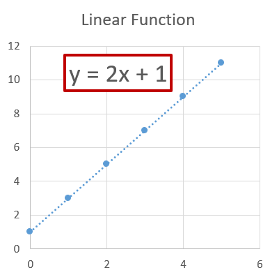
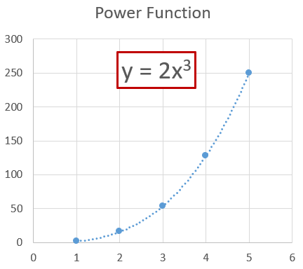
In science there are many types of functions, and general chemistry makes extensive use of three types; linear, power and exponential.

1. Linear Function:
\[y=mx+b\]

2. Power Function:
\[y=ax^m \]

(which is linear in the logarithmic form)

\[logy =mlogx + loga\]

3. Exponential Function:

\[y=ae^{mx}\]

(which is linear for a plot of the natural log of the dependent variable against the independent variable)

\[ lny=mx+lna\]

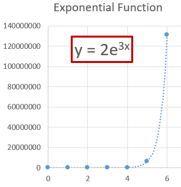Figure \(\PageIndex{2}\): Plots of the three types of functions that are commonly used in general chemistry.

We will not use the power function or exponential function until the second semester of general chemistry, when students will be using these extensively. There is a review of logarithms in the prelude to Chapter 14, and this Chapter we will only cover linear functions.

Graphing Linear Functions

Equation 1B.5.3 is a linear equation \[y=mx+b\nonumber \]

m is called the slope of the line, which is the ratio of the change in y (the rise) to the change in x (the run). Since the line is linear, the slope is the same between any two points along the line.
b is called the y-intercept, which is the value of y when x=0.

Steps for Graphing a Linear Function

Pick your range and scale: In graphing a linear function the first step is to identify the range and scale for each axes. The range is defined by the minimum and maximum value along each of the axes. The scale is defined by the values of each line in the grid, which is used both to plot the data points, and once graphed, to read values from the graph. There are often minor and major marks given to the grid, where the major marks show the numerical value of that position.

Choosing the Range: There are two approaches. The first is to use the highest and lowest data value as the lower and upper bound of the range, although you may want the actual bounds to be some easy number to read, like a multiple of ten. The second approach is to look at the data, and see if the data is bounded by some real limit. For example, in the above data we are looking at the solubility of a salt in liwuid water, so the temperature range may want to be defined by the temperature range where water is a liquid, even if your highest data point is not at the boiling point, and your lowest is not at the freezing point.
Choosing the Scale: Here you want the grid line to be easy to read. If possible, multiple's of 10 are very useful, but you need to look at the data. Want you want to avoid is where each mark is some hard to read value.

Plot data: Mark each data point on the graph (like in Figure 1B.5.1, but do not write down the x,y coordinate values, just mark a point on the graph to indicate where there is a data value.
Hand draw a best fit line that has an even distribution of points on both sides of the line. If the data is truly a linear function, there will be a random distribution of points along the line. Figure 1b.5.3 shows such a "best fit line".

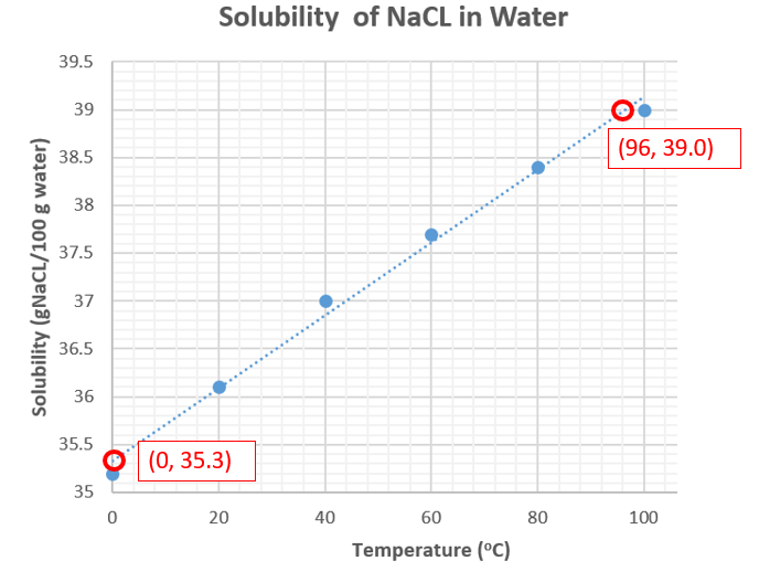
Figure \(\PageIndex{3}]): Best fit line that evenly describes the data. Not we do not connect the points, and some of the points are not on the line.
Pick two points to calculate the slope from. Start at the left side and find the point on the line with the smallest values where the line crosses the grid lines, here it is point (0,25.50), and then starting at the right end pick the point with the highest values (96,39.00).

Note the precision is defined by both the data and the scale on the grid lines.
- For the y-axis the precision is defined by the data, and although we have a mark every 0.1 values, so it looks like we could report solubility to the .01 value, the original data was only known to the 0.1 value (table 1B.5.1). So so even though the scale on the graph is more precise, we can only use that precision to read from the scale, and not report the value. That is from the scale we could read to a value of 35.30 and not 35.3, but we must use 35.3 in our calculation
- For the x-axis the original data has a precision to the 0.1 digit, that is, we have values like 20.0 ^oC. But the smallest value on the minor grid axis is 4 ^oC, and so we have to "guess" between them to report the uncertainty, and thus choose the precision to be to the "ones" position.
Note, if we choose points near to each other, we can lose significant digits. For example, if the second point was (4,35.5) the change in temperature would be 4-0 or 4 degrees (1 significant digit), while using the value on the graph give 96-0, or 96 degrees, which has two significant Figures.
That is, we report all certain, and the first uncertain data point, as read off the graph. A graph scale should never have a smaller scale than the raw data, that is, it can't add to the precision

Now calculate the slope

\[\text{slope} = m=\frac{\text{rise}}{\text{run}} = \frac{\left( y_2 - y_1 \right)}{\left( x_2 - x_1 \right)} =\frac{\left( S_2 - S_1 \right)}{\left( T_2 - T_1 \right)} =\frac{\left( 39.0 -35.3 \right)}{\left( 96 - 0 \right)} = {\color{blue}0.039 \:\frac{g\; NaCl}{100gH_2O\cdot \; ^oC}}\]
Now calculate the y intercept. Since the graph goes through zero, you can just read it from the graph

Since the x-axis includes zero, you can simply read it from the graph, b=35.3(gNaCl/100g water).
If your graph does not include the zero point, you can extrapolate backwards from a given value.
We know that:
\[m=\frac{\Delta{y}}{\Delta{x}} = \frac{\Delta{S}}{\Delta{T}} \]

If we define S₂₀=solubility when T=20, and S₀=solubility when T=0, then b= S₀, and S₂₀comes from the graph on Figure 1B.5.3 where, S₂₀=36.1(gNaCl/100g water).

\[{\color{blue}m}=\frac{\textcolor{red}{S_{20}}-S_{0}}{20-0}= \frac{\textcolor{red}{S_{20}}-b}{\Delta{T}_{(=20)}}\]

Where \(\Delta{T_{(=20)}}\) means the value of \(\Delta T\)= 20,

solving for b and including units in numerical calculation gives:

\[b={\color{Red} S_{20}}-\textcolor{blue}{m}(\Delta{T}_{(=20)})={\color{red}36.1\left (\frac{g\; NaCl}{100gH_2O} \right )}- {\color{blue}0.039 \:\frac{g\; NaCl}{100gH_2O\cdot \; ^oC}}\left ( 20 \; ^oC\right )=35.3\left (\frac{g\; NaCl}{100gH_2O} \right )\]

Temperature Scales

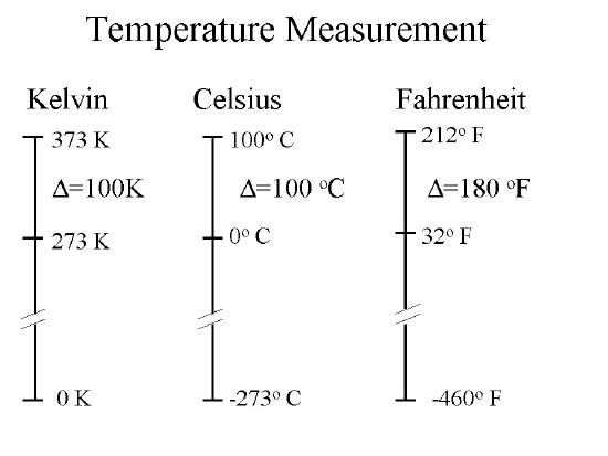
There are three temperature scales you need to be familiar with, Celsius, Kelvin and Fahrenheit. It should also be noted that the term temperature is used in two contexts, the actual temperature of an object, or the temperature change an object undergoes. As we shall see, the temperature of an object in Celsius is different than in Kelvin, but a temperature change in Celsius equals the temperature change in Kelvin.

Kelvin Scale

The kelvin Scale, which is one of the 7 SI base units, and is now defined by four of the SI defining constants (k, h,c & Δν_Cs). Kelvin is a thermodynamic temperature scale, and the lowest possible temperature is 0K, absolute zero.

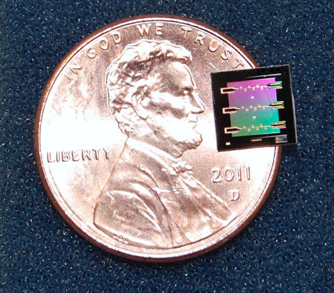
\(\PageIndex{1}\): Scientists at NIST cooled a "micro drum" fabricated on a sapphire chip like the one on this penny to the lowest possible energy of the "quantum ground state", which was below 400 \(\mu\) kelvin.

Celsius Scale

The Celsius scale is named after the Swedish astronomer Anders Celsius, who in 1742 created a temperature scale based on the normal (1 atm) melting and boiling points of water. The original Celsius thermometer actually had the boiling point at 0 deg C and the freezing point at 100. A year later this was reversed, with zero being the freezing point and 100 being the boiling point. This early scale was often called the centigrade scale as there were 100 degrees between the normal (1 atm) freezing and boiling points. Today, this is not a valid definition, and the degree Celsius is defined by the Kelvin scale, where the normal boiling point of water (at 1 atm pressure) is 273.15K.

\[T_{Celsius}=T_{kelvin} + 273.15\]

Fahrenheit Scale

This scale was introduced in 1724 by Daniel Gabriel Fahrenheit and there are several stories on how this scale originated, but zero was essentially defined by how cold a salt water solution could be lowered (salt lowers the freezing point of water), and 96 degrees was defined by the human temperature. In 1776 this scale was redefined by two exact points, 32 degrees being the freezing point of water, and 212 being the boiling point.

Temperature Conversions

Figure 1B.3.2 shows the relationship between the three commons scales with values given for absolute zero and the boiling and freezing points of water.

Figure \(\PageIndex{2}\): Relationship of the three common temperature scales

Celsius/Kelvin Conversions

Because the kelvin defines the Celsius scale, the conversion is simple.

Celsius to kelvin

\[T_{Celsius}=T_{kelvin} + 273.15\]

Kelvin to Celsius

\[T_{kelvin}=T_{Celsius} - 273.15\]

Celsius/Fahrenheit

Both Celsius and Fahrenheit are linear scales and a plot of data from the freezing point to the boiling point of water can show the relationship. In Figure 1B.3.3 we plot the Fahrenheit values along the ordinate (y-axis) and Celsius along the abscissa (x-axis) and we note there are multiple ways of writing the equation relating Celsius and Fahrenheit.

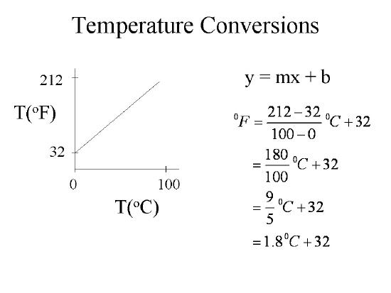
Figure \(\PageIndex{3}\): plot of T(F) as a function of T(C)

We note that the above equation has two forms

Celsius to Fahrenheit

\[T_F=1.8T_C+32\]

Fahrenheit to Celsius

\[T_C=\frac{T_F-32}{1.8}\]

These equations are much more complicated than the density equation because the y-intercept is not zero. In the following videos we will develop a quick technique for converting between these temperature scales called the Plus 40/minus 40 technique. So first, lets look at the difference between the linear plots of Fahrenheit vs. Celsius and mass vs. volume.

So what we do is find the temperature at which T_F= T_C and make that value equal to zero

Exercise \(\PageIndex{1}\)

At what temperature does T_F= T_C?

Answer

We start by setting them equal to a common T,

\[T_F =T_C=T \nonumber\]

Then substitute into the equation and solver for T

\[T=\frac{9}{5}T+32 \\ T(1-\frac{9}{5})=32 \\ T(\frac{-5}{5})=32 \\ T=32(\frac{-5}{4}) \\ T=-40 \nonumber\]

So the scales converge at -40 degrees.

Plus Forty/Minus Forty Technique

The strategy of the plus forty/minus forty techniques is to make the value where the two scales intersect equal to forty, then the y-intercept is zero, and so you can just multiple or divide by the slope. This is a three step process

Add 40 to the number (since the intersected at -40, that value is now zero)
multiple or divide by the slope
- If going from Fahrenheit to Celsius, divide by 1.8
- If going from Celsius to Fahrenheit, multiply by 1.8
Subtract the 40If going from Fahrenheit to Celsius, divide by 1.8

This technique is explained in the following video.

Plus forty/minus forty explained

This video derives the plus forty/minus forty technique

Derivation of the plus forty/minus forty technique

Video \(\PageIndex{2}\): Graphing Part 2: temperature conversions

Example \(\PageIndex{7}\): Celsius to Fahrenheit

Convert 184K to Fahrenheit

Solution

Note, this video needs to be redone when I get back to AR, as I forgot to write down the negative sign (although I stated it), and the date was wrong, as it was really 1983.

Ans: -128ºF

Video \(\PageIndex{3}\): Temperature conversion Plus 40 minus 40 method (C to F)

Exercise \(\PageIndex{1}\)

Add exercises text here.

Answer: Add texts here. Do not delete this text first.

Example \(\PageIndex{8}\): Fahrenheit to Celsius

136 ºF =? ºC

Solution

58ºF

Video \(\PageIndex{4}\): Temperature conversion Plus 40 minus 40 method (F to C)

Test Yourself

Query \(\PageIndex{1}\)

Contributors and Attributions

Robert E. Belford (University of Arkansas Little Rock; Department of Chemistry). The breadth, depth and veracity of this work is the responsibility of Robert E. Belford, rebelford@ualr.edu. You should contact him if you have any concerns. This material has both original contributions, and content built upon prior contributions of the LibreTexts Community and other resources, including but not limited to:

Ronia Kattoum (Learning Objectives)
Elena Lisitsyna (H5P interactive modules)