6.2.3: H2O

Construct SALCs and the molecular orbital diagram for H\(_2\)O.

This is the first example so far that is not a linear molecule. Water is a bent molecule, and so it is important to remember that interactions of pendant ligands are dependent on their positions in space. You should consider the positions of the three atoms in water to be essentially fixed in relation to each other. The process for constructing the molecular orbital diagram for a non-linear molecule, like water, is similar to the process for linear molecules. We will walk through the steps below to construct the molecular orbital diagram of water.

Preliminary Steps

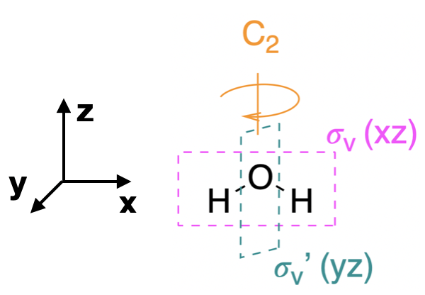
Step 1. Find the point group of the molecule and assign Cartesian coordinates so that z is the principal axis.

The H\(_2\)O molecule is bent and its point group is \(C_{2v}\). The \(z\) axis is collinear with the principal axis, the \(C_2\) axis. There is no need to simplify this problem, as we had done for previous examples. The \(C_{2v}\) point group is simple enough.

Figure \(\PageIndex{1}\): The water molecular is in the \(C_{2v}\) point group. (CC-BY-NC-SA; Kathryn Haas)

Step 2. Identify and count the pendant atoms' valence orbitals.

Each of the two pendant hydrogen atoms has one valence orbital, the \(1s\). Thus, we can expect a total of two SALCs from these two atoms.

Generate SALCs

The SALCs for H\(_2\)O are quite simple, yet we will systematically derive the SALCs here to demonstrate the process.

Step 3. Generate the \(\Gamma\)'s

Use the \(C_{2v}\) character table to generate one reducible representation (\(\Gamma\)); in this case we need only one \(\Gamma\) because there is only one type of valence orbital (the \(1s\)). For each \(s\) orbital, assign a value of 1 if it remains in place during the operation or zero if it moves out of its original place. The \(\Gamma\) is given below:
\[\begin{array}{|c|cccc|} \hline \bf{C_{2v}} & E & C_2 &\sigma_v (xz) & \sigma_v' (yz) \\ \hline \bf{\Gamma_{1s}} & 2 & 0 & 2 & 0 \\ \hline \end{array} \nonumber \]

Step 4. Break \(\Gamma\)'s into irreducible representations for individual SALCs

Reduce each \(\Gamma\) into its component irreducible representations. Using either of the processes described previously, we find that the \(\Gamma\) reduces to the two irreducible representations \(A_1\) and \(B_1\) under the \(C_{2v}\) point group.

\[\begin{array}{|c|cccc|} \hline \bf{C_{2v}} & E & C_2 &\sigma_v (xz) & \sigma_v' (yz) \\ \hline \bf{\Gamma_{1s}} & \bf 2 & \bf 0 & \bf 2 & \bf 0 \\
A_{1} & 1 & 1 & 1 & 1 \\
B_{1} & 1 & -1 & 1 & -1 \\
\hline \end{array} \nonumber \]

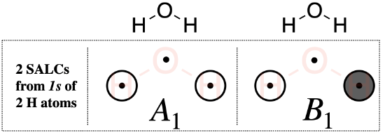
Step 5. Sketch the SALCs

From the systematic process above, you have found the symmetries (the irreducible representations) of both SALCs under the \(C_{2v}\) point group. To sketch the SALC that corresponds to each irreducible representation, again we use the \(C_{2v}\) character table, and specifically the functions listed on the right side columns of the table.

One \(A_1\) SALC: The \(A_1\) SALC is singly degenerate and symmetric with respect to both the principle axis (\(z\)) and the inversion center (\(i\)) (based on its Mulliken Label). We can look at the functions in the \(C_{2v}\) character table that correspond to \(A_1\) and see that it is completely symmetric under the group (because the combination of \(x^2,y^2,z^2\) shows that it is totally symmetric). This would be the same symmetry as an \(s\) orbital on the central oxygen atom. From this information, we know that this SALC must have symmetry compatible with an \(s\) orbital on the central atom. We can also see from the character table that the \(z\) axis, and thus a \(p_z\) orbital on oxygen, also possesses \(A_1\) symmetry. This tells us that in addition to being compatible with the oxygen \(s\) orbital, it should also be compatible with the oxygen \(p_z\) orbital. From this information we can draw the \(A_1\) SALC shown in Figure \(\PageIndex{2}\). If it is not obvious how the \(A_1\) sketch in Fig. \(\PageIndex{2}\) is compatible with the \(s\) and \(p_z\) orbitals of oxygen, inspect the drawings corresponding to molecular orbitals \(2a_1\) and \(3a_1\) in Fig. \(\PageIndex{3}\).

One \(B_{1}\) SALC: The Mulliken Label tells us that the \(B_{1}\) SALC is singly degenerate and antisymmetric with respect to both the principal axis and the inversion center. The function, \(x\), appearing with \(B_{1}\) in the character table tells us that this SALC has the same symmetry as the \(x\) axis, or a \(p_x\) orbital on the central oxygen atom. From this information, we know that this SALC should be compatible with a \(p_x\) orbital on the central atom, and we can draw the \(B_{1}\) SALCs shown in Figure \(\PageIndex{2}\). If it is not obvious how the \(B_1\) sketch in Fig. \(\PageIndex{2}\) is compatible with the \(p_x\) orbital of oxygen, inspect the drawing corresponding to molecular orbital \(1b_1\) in Fig. \(\PageIndex{3}\).

Figure \(\PageIndex{2}\): Sketch of the \(A_1\) and \(B_1\) hydrogen SALCs of water. (CC-BY-NC-SA; Kathryn Haas)

Not convinced about the sketches of these SALCs? You can convince yourself by putting them to the test. Try the exercise below.

Exercise \(\PageIndex{1}\)

Perform all operations of the \(C_{2v}\) point group on the two sketches of H SALCs shown in Figure \(\PageIndex{2}\), and convince yourself that each sketch does possess the \(A_1\) and \(B_1\) symmetries assigned to them, respectively, under the \(C_{2v}\) point group.

Answer

Add texts here. Do not delete this text first.

Draw the MO diagram for \(H_2O\)

Step 6. Combine SALCs with AO’s of like symmetry.

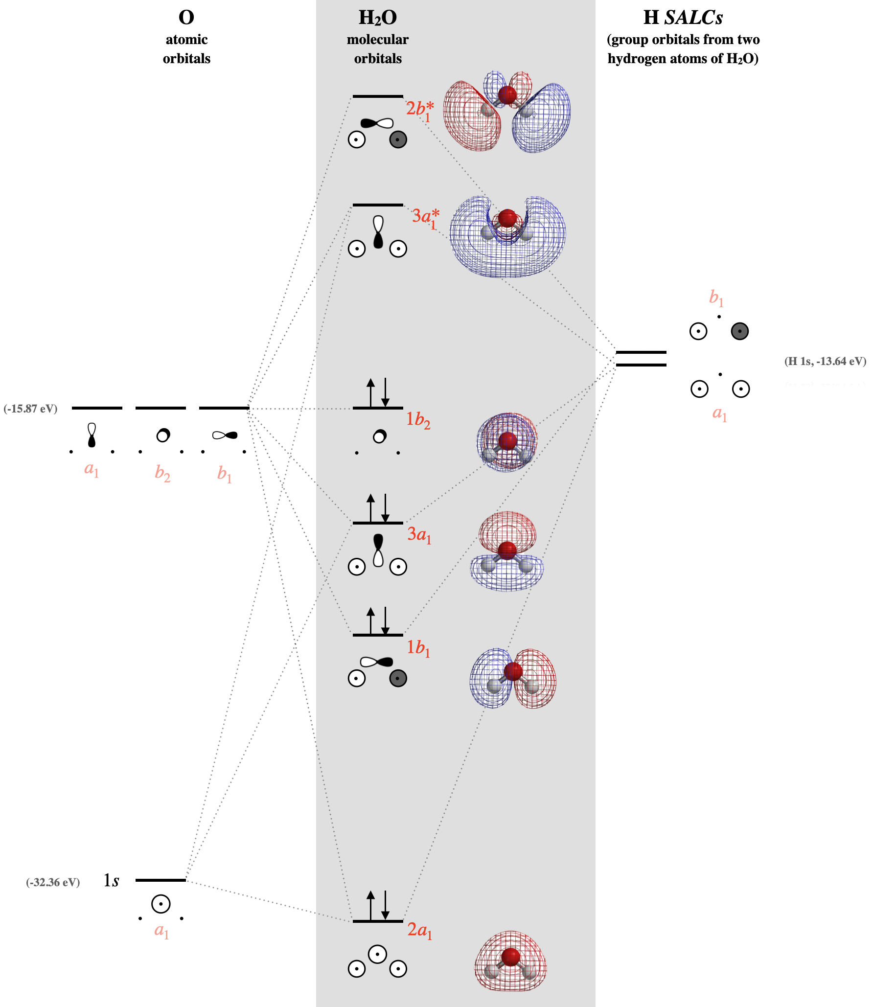
First we must identify the valence orbitals on the central oxygen: there are four including \(2s\), \(2p_x\), \(2p_y\), and \(2p_z\). Now we identify the symmetry of each using the \(C_{2v}\) character table. The symmetry of a central \(2s\) orbital corresponds to the combination of functions \(x^2\), \(y^2\), and \(z^2\) in the character table; this is \(A_1\). The \(p_z\) orbital also corresponds to \(A_1\). And so on... The symmetries of oxygen valence orbitals are listed below. \[2s =A_1 \\ 2p_x = B_1 \\ 2p_y = B_2 \\ 2p_z = A_1 \nonumber \]

Now that we have identified the symmetries of the two hydrogen SALCs and the four valence orbitals on oxygen, we know which atomic orbitals and SALCs may combine based on compatible symmetries. We also need to know the relative orbital energy levels so that we can predict the relative strength of orbital interactions. The orbital ionization energies are listed in Section 5.3.1.

With knowledge of both orbital symmetries and energies, we can construct the molecular orbital diagram. The valence orbitals of oxygen go on one side of the diagram while the hydrogen group orbitals are drawn on the opposite side. Molecular orbitals are drawn in the center column of the diagram, as shown in Figure \(\PageIndex{3}\):

Figure \(\PageIndex{3}\): The molecular orbital diagram of water. Molecular orbital surfaces calculated using Spartan software. The surface of the \(3a_1^*\) orbital has been trimmed. (CC-BY-NC-SA; Kathryn Haas)

Example \(\PageIndex{1}\)

In the previous examples shown for the molecular orbital diagrams of the bifluoride anion and carbon dioxide, we discussed differences in the understanding of those molecules from molecular orbital theory compared to Lewis structures. Water contains two lone pairs in its Lewis structure. Compare the predictions about water's lone pairs of electrons and its reactivity based on (1) the combination of elementary models (Lewis, Valence Bond, and Hybridized Orbital theories) and (2) Molecular Orbital theory. Specifically address and explain how the elementary models differ from molecular orbital theory in the following respects:

1. Where are the lone pairs in water?
2. Are the two lone pairs equivalent or are they different?
3. Where are sites on the molecule that will undergo reaction with electrophiles and nucleophiles?

Solution

1) Elementary models: The Lewis structure predicts that two lone pairs are (a) localized on the oxygen atom of water and that (b) both lone pairs are equivalent. The Lewis structure, combined with Valence Bond Theory, would predict that lone pairs occupy two equivalent hybridized \(sp^3\) atomic orbitals on oxygen. (c) Lewis theory would predict that the oxygen lone pairs are nucleophiles; thus an electrophile would react with the oxygen atom lone pairs. The polarized O-H bond leaves the H atoms as the most electrophilic locations on the water molecule; thus nucleophiles would react at the H atoms of water.

2) Molecular orbital theory: The molecular orbitals predict that (a) the two lone pairs of water are not equivalent, and that (b) each is distributed over the entire molecule. One lone pair is in the truly non-bonding \(1b_2\) orbital (Figure \(\PageIndex{3}\)), which is also the HOMO. There is not another truly non-bonding orbital in the molecule, but the lowest-energy \(2a_1\) orbital could be considered mostly non-bonding due to the large energy difference between it and other valence orbitals. (c) Although the \(2a_1\) orbital can be considered mostly non-bonding, we cannot expect the electrons in \(2a_1\) to react readily, as they are in the lowest-energy molecular orbital. Molecular orbital theory predicts that reactions occur at the HOMO and LUMO orbitals. The HOMO reacts with electrophiles, and in this case, the HOMO is distributed over the top and bottom faces of the molecule, and is centered on the oxygen atom. The LUMO would react with nucleophiles. The LUMO is the orbital labeled \(3a_1^*\) in Figure \(\PageIndex{3}\), and has a major lobe that is distributed more heavily over the H atoms, and from this we should predict H atoms to be the preferred site of reaction for nucleophiles.

Expressing molecular orbitals in terms of \(\Psi\)

The general expression for a molecular orbital, or the linear combination of atomic orbitals (LCAO), was given previously as \(\Psi=c_{a} \psi_{a}+c_{b} \psi_{b}\). In this expression, the wavefunction of two atoms (\(\psi_a\) and \(\psi_b\)) is combined to form the wavefunction of the molecular orbital. The coefficients \(c_a\) and \(c_b\) quantify the contribution of each atomic \(\psi\) to the molecular \(\Psi\).

\[\Psi=c_{a} \psi_{a}+c_{b} \psi_{b} \nonumber \]

In the case of polyatomic orbitals, each LCAO is constructed of atomic orbitals from a central atom and group orbitals (SALCs) from the pendent atoms. In the case of water, the expression above could be modified to give the expression below.
\[\Psi = c_{oxygen}\left(\psi_{oxygen}\right) + c_{SALCs}\left(N (\psi_{H_a} \pm \psi_{H_b})\right) \nonumber \]
N represents the normalizing requirement that was mentioned previously in reference to the requirements for electron wavefunctions and probability functions. The normalizing requirement simply stated is the requirement that the probability of finding the electron in any orbital, including group orbitals, is 1. In general, the value of N for a group orbital is... \[N=\frac{1}{\sum{c_i^2} } \nonumber \] ...where \(c_i\) is the coefficient of each unique atomic orbital that contributes to the group. For the hydrogen SALCs of water, there are two atomic orbitals that contribute to equally to each SALC, and so the coefficient on each of the two orbitals is 1. This gives \(N=\left(\frac{1}{\sqrt{1^2 + 1^2}}\right) = \frac{1}{\sqrt{2}}\) for the H SALCs of water.

There are only two hydrogen SALCs: the one in which the hydrogen wavefunctions are added (\(N(\psi_{H_a} + \psi_{H_b})\)) has \(A_1\) symmetry, and the one in which the hydrogen wavefunctions are subtracted (\(N(\psi_{H_a} - \psi_{H_b})\)) has \(B_1\) symmetry.

The molecular orbitals from Figure \(\PageIndex{3}\) are expressed below in terms of their LCAO of individual wavefunctions. Yet, note that these expressions are simplifications that ignore orbital mixing. For example, as expressed below, they ignore contributions of oxygen \(2s\) to the higher energy moelcular orbitals with \(A_1\) symmetry (the \(3a_1\) and \(3a_1^*\) in Figure \(\PageIndex{3}\)).

\[\begin {array}{|rcccc|l|}
\hline MO & & Oxygen AO & & Hydrogen SALC & Description \\
\hline \Psi_{2a_1} & = & c_{(ox1)}\psi_{(2s)} & + & c_{(hy1)} [N(\psi_{H_a} + \psi_{H_b})] & c_{(hy1)} \text{ is positive; bonding, slightly nonbonding} \\
\Psi_{1b_1} & = & c_{(ox2)}\psi_{(2p_x)} & + & c_{(hy2)} [N(\psi_{H_a} - \psi_{H_b})] & c_{(hy2)} \text{ is positive; bonding} \\
\Psi_{3a_1} & = & c_{(ox3)}\psi_{(2p_z)} & + & c_{(hy3)} [N(\psi_{H_a} + \psi_{H_b})] & c_{(hy3)} \text{ is positive; bonding} \\
\Psi_{1b_2} & = & \psi_{(2p_y)} & & & \text{nonbonding} \\
\Psi_{3a_1}^* & = & c_{(ox4)}\psi_{(2p_z)} & + & c_{(hy4)} [N(\psi_{H_a} + \psi_{H_b})] & c_{(hy4)} \text{ is negative; antibonding} \\
\Psi_{1b_1}^* & = & c_{(ox5)}\psi_{(2p_x)} & + & c_{(hy5)} [N(\psi_{H_a} - \psi_{H_b})] & c_{(hy5)} \text{ is negative; antibonding} \\
\hline \end {array} \nonumber \]