7.1.1: Tetrahedral and Octahedral Geometries

Saint Mary's College: CHEM 342
Bioinorganic Chemistry
Spring 2020: Dr. Kathryn Haas

Agenda   ●   Readings   ●  Worksheets   ●  Essays  ●  WiSEWIKI

---

Until this point, we have focused on one of the most common cases for metal complexes, the 6-coordinate octahedral ligand field geometry. Now, we will examine other geometries, with a focus on 4-coordinate ligand fields. Almost everything you have already learned about octahedrons can be applied to 4-coordinate metal complexes (effects of metal and ligands on \(\Delta\)); the main difference is the splitting pattern of d-orbitals is different in each 4-coordinate complex than it was in the octahedral cases. Also, the magnitudes of splitting are different in important ways.

Since CFT is simpler than LFT, let's use CFT to describe and derive these "new-to-you" splitting patterns. Now is a good time to go back and recall how CFT was used to derive the splitting of d-orbitals in an octahedral field so that you can use that as a launching pad for deriving the tetrahedron (harder) and square planar geometries:

Exercise \(\PageIndex{1}\)

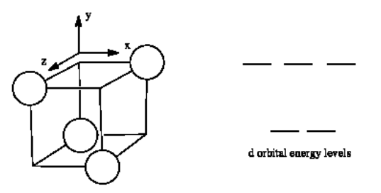
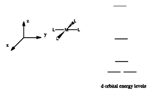
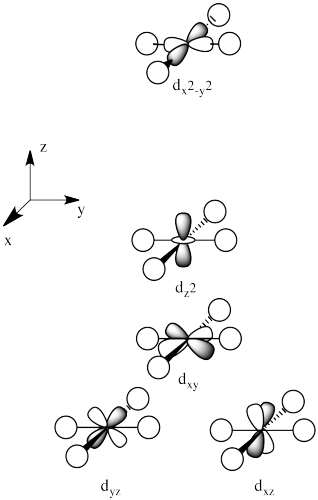
The d orbital splitting diagram for a tetrahedral coordination environment is shown below. Given this diagram, and the axes in the accompanying picture, identify which d orbitals are found at which level. In the picture, the metal atom is at the center of the cube, and the circle represent the ligands.

Figure \(\PageIndex{1}\):

Answer

The three upper orbitals (dy, dx, dz) interact a little more strongly with the ligands. The two lower orbitals (dz² and dx²-y²) interact a little more weakly.

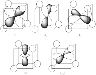The reason for the difference in the interaction has to do with how close the nearest lobe of a d orbital comes to a ligand. There are really two possible positions: the face of a cube or the edge of a cube. If the ligands are at alternating corners of the cube, then the orbitals pointing at the edges are a little closer than those pointing at the faces of the cube.

Exercise \(\PageIndex{2}\)

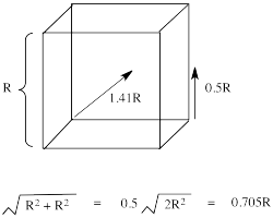
Typically, the d orbital splitting energy in the tetrahedral case is only about 4/9 as large as the splitting energy in the analogous octahedral case. Explain why it is smaller for the tetrahedral case.

Answer

The ligands do not overlap with the d orbitals as well in tetrahedral complexes as they do in octahedral complexes. Thus, there is a weaker bonding interaction in the tetrahedral case. That means the antibonding orbital involving the d electrons is not raised as high in energy, so the splitting between the two d levels is smaller.

Exercise \(\PageIndex{3}\)

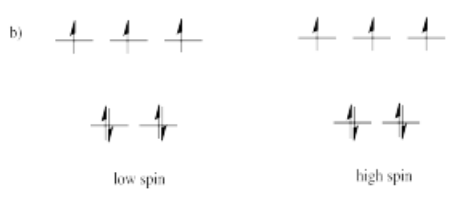
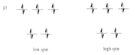
Suppose each of the ions below were in tetrahedral coordination environments. Draw the d orbital diagrams for the high-spin and the low-spin case for each ion. Which one (high-spin or low-spin) is more likely?

a) Mn²⁺ b) Co²⁺ c) Ni²⁺ d) Cu⁺ e) Fe³⁺ f) Cr²⁺ g) Zn²⁺

Answer a)

High spin is more likely for tetrahedral coordination geometry due to weak interactions between ligand orbitals and metal d-orbitals.

Answer b)

High spin is more likely for tetrahedral coordination geometry due to weak interactions between ligand orbitals and metal d-orbitals.

Answer c)

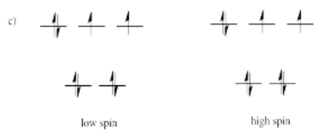
High spin is more likely for tetrahedral coordination geometry due to weak interactions between ligand orbitals and metal d-orbitals.

Answer d)

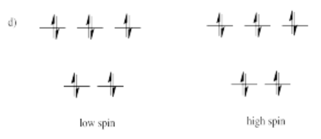
High spin is more likely for tetrahedral coordination geometry due to weak interactions between ligand orbitals and metal d-orbitals.

Answer e)

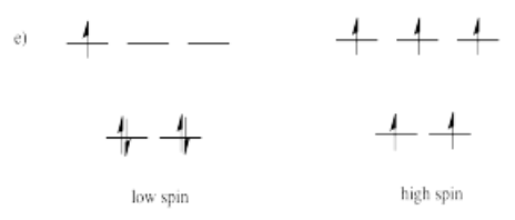
High spin is more likely for tetrahedral coordination geometry due to weak interactions between ligand orbitals and metal d-orbitals.

Answer f)

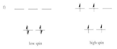
High spin is more likely for tetrahedral coordination geometry due to weak interactions between ligand orbitals and metal d-orbitals.

Answer g)

High spin is more likely for tetrahedral coordination geometry due to weak interactions between ligand orbitals and metal d-orbitals.

Exercise \(\PageIndex{4}\)

Usually, tetrahedral ions are high spin rather than low spin. Explain why.

Answer

Because the d orbital splitting is much smaller in the tetrahedral case, it is likely that the energy required to pair two electrons in the same orbital will be greater than the energy required to promote an electron to the next energy level. In most cases, the complex will be high spin.

Exercise \(\PageIndex{5}\)

The d orbital splitting diagram for a square planar environment is shown below. Given this diagram, and the axes in the accompanying picture, identify which d orbitals are found at which level.

Figure \(\PageIndex{18}\):

Answer

The orbitals are shown in order of energy.

Exercise \(\PageIndex{6}\)

Predict whether each compound will be square planar or tetrahedral.

a. [Zn(NH₃)₄]²⁺

b. [NiCl₄]²⁺

c. [Ni(CN)₄]^2-

d. [Ir(CO)(OH)(PCy₃)₂]²⁺ ; Cy = cyclohexyl

e. [Ag(dppb)₂]⁺ ; dppb = 1,4-bis(diphenylphosphino)butane

f. PtCl₂(NH₃)₂

g. PdCl₂(NH₃)₂

h. [CoCl₄]^2–

i. Rh(PPh₃)₃Cl

Answer a)

[Zn(NH₃)4] ²⁺ 3d metal, d¹⁰, sigma donor ligand → tetrahedral

Answer b)

[NiCl₄] ²⁺ 3d metal, d⁸, pi donor ligand → tetrahedral

Answer c)

[Ni(CN)₄] ^2- 3d metal, d⁸, pi acceptor ligand → square planar

Answer d)

[Ir(CO)(OH)(PCy₃)₂] ²⁺ 5d metal, d⁸ → square planar

Answer e)

[Ag(dppb)₂]¹⁺ 4d metal, d¹⁰, sigma donor ligand → tetrahedral

Answer f)

[PtCl₂(NH₃)₂] 5d metal, d⁸ → square planar

Answer g)

[PdCl₂(NH₃)₂] 4d metal, d⁸, M⁺², sigma donor ligand → square planar

Answer h)

[CoCl₄] ^2– 3d metal, d⁷, sigma donor ligand → tetrahedral

Answer i)

[Rh(PPh₃)₃Cl] 5d metal, d⁸ → square planar

LFSE and SE for Other Geometries

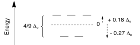
Just like in the case of octahedral metal complexes, we can apply CFT (or LFT) to calculate LFSE and SE of 4-coordinate (or any-coordinate) metal complexes. Once again, in terms of the d orbital splitting diagram, the results are similar to what we see from molecular orbital theory. For tetrahedral geometry, which is the most common geometry when the coordination number is four, we get a set of two high-lying orbitals and three lower ones.

Figure \(\PageIndex{11}\):

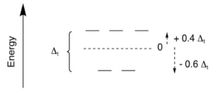
The overall splitting is expressed as Δ_t; the t stands for tetrahedral. However, sometimes it is useful to compare different geometries. In crystal field theory, it can be shown that the amount of splitting in a tetrahedral field is much smaller than in an octahedral field. In general, Δ_t = 4/9 Δ_o.

Figure \(\PageIndex{12}\):

Which geometries are most likely?

We wouldn't usually use crystal field theory to decide whether a metal is more likely to adopt a tetrahedral or an octahedral geometry. In most cases, the outcome is more strongly dependent on factors other than the d orbital energies. For example, maybe a complex would be too crowded with six ligands, so it only binds four; it becomes tetrahedral rather than octahedral. Or maybe a metal does not have enough electrons in its valence shell, so it binds a couple more ligands; it becomes octahedral rather than tetrahedral.

However, this comparison between Δ_o and Δ_t does help to explain why tetrahedral complexes are much more likely than octahedral complexes to adopt high-spin configurations. The splitting is smaller in tetrahedral geometry, so pairing energy is more likely to become the deciding factor there than it is in octahedral cases.

Exercise \(\PageIndex{1}\)

Tetrahedral complexes are pretty common for high-spin d⁶ metals, even though the 18-electron rule suggests octahedral complexes should form. In contrast, low-spin d⁶ complexes do not usually form tetrahedral complexes. Use calculations of stabilisation energies to explain why.

Answer

high-spin d⁶

octahedral

SE = [2(0.6) -4(0.4)]Δ_o + PE

SE = -0.4Δ_o + PE

tetrahedral

SE = [3(0.4) - 3(0.6](4/9)Δ_o + PE

SE = -0.6Δ_o + PE

ΔSE = SE_oh - SE_td = -0.4Δ_o + PE -(-0.6Δ_o + PE) = +0.2Δ_o

This is a slight preference for tetrahedral.

low-spin d⁶

octahedral

SE = [0(0.6) -6(0.4)]Δ_o + 3PE

SE = -2.4Δ_o + 3PE

tetrahedral

SE = [2(0.4) - 4(0.6](4/9)Δ_o + 2PE

SE = -1.6Δ_o + PE

ΔSE = SE_oh - SE_td = -2.4Δ_o + 3PE -(-1.6Δ_o + 2PE) = -0.8Δ_o + PE

This is a preference for octahedral, although it would be offset by the pairing energy.

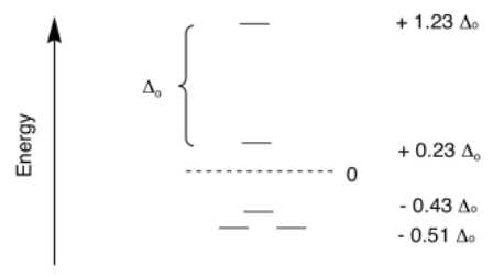
Crystal field theory has also been used to determine the splitting between the orbitals in a square planar geometry. That is a much more complicated case, because there are four different levels. Once again, the energy levels are often expressed in terms of Δ_o.

Figure \(\PageIndex{13}\):

We could use a calculation of stabilisation energy to predict whether a particular complex is likely to adopt a tetrahedral or a square planar geometry. Both geometries are possible, so it would be useful to be able to predict which geometry occurs in which case. However, just as in the case of comparing octahedral and tetrahedral gemoetries, there is another factor that is often more important.

Figure \(\PageIndex{14}\):

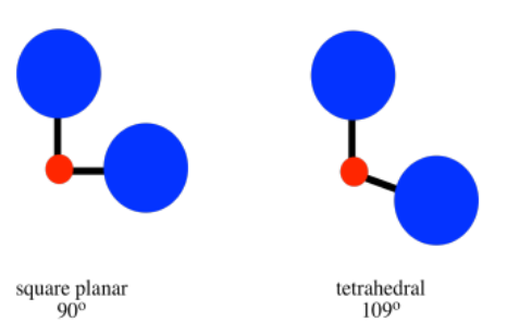
That factor is steric crowding. In a tetrahedron, all the ligands are 109^o from each other. In a square planar geometry, the ligands are only 90^o away from each other. Tetrahedral geometry is always less crowded than square planar, so that factor always provides a bias toward tetrahedral geometry. As a result, we might expect square planar geometry to occur only when sterics is heavily outweighed by ligand field stabilisation energy.

Exercise \(\PageIndex{2}\)

The most common examples of square planar complexes have metals that are d⁸. Use calculations of the stabilisation energy to explain why if the complex is:

(a) low-spin

(b) high-spin

Answer a)

high-spin d⁸

square planar

SE = [1.23 + 0.23 - 2(0.43) -4(0.51)]Δ_o + 3PE

SE = -1.44Δ_o + 3PE

tetrahedral

SE = [4(0.4) - 4(0.6](4/9)Δ_o + 3PE

SE = -0.36Δ_o + 3PE

ΔSE = SE_sq - SE_td = -1.44Δ_o + 3PE -(-0.36Δ_o + 3PE) = -1.08Δ_o

This is an appreciable preference for square planar.

Answer b)

low-spin d⁸

square planar

SE = [0 + 2(0.23) - 2(0.43) -4(0.51)]Δ_o + 4PE

SE = -2.44Δ_o + 4PE

tetrahedral = same as before (ls = hs for d⁸ tetrahedral)

ΔSE = SE_sq - SE_td = -2.44Δ_o + 3PE -(-0.36Δ_o + 3PE) = -2.08Δ_o + PE

This is an even more appreciable preference for square planar, although it is offset by pairing energy. Pairing energy would have to be twice as big as Δ_o in order to completely offset the LFSE.

Attribution

Chris P Schaller, Ph.D., (College of Saint Benedict / Saint John's University)