0.1.1: Review of Orbital Shapes

Last updated
Save as PDF

Page ID: 190489

\( \newcommand{\vecs}[1]{\overset { \scriptstyle \rightharpoonup} {\mathbf{#1}} } \) \( \newcommand{\vecd}[1]{\overset{-\!-\!\rightharpoonup}{\vphantom{a}\smash {#1}}} \)\(\newcommand{\id}{\mathrm{id}}\) \( \newcommand{\Span}{\mathrm{span}}\) \( \newcommand{\kernel}{\mathrm{null}\,}\) \( \newcommand{\range}{\mathrm{range}\,}\) \( \newcommand{\RealPart}{\mathrm{Re}}\) \( \newcommand{\ImaginaryPart}{\mathrm{Im}}\) \( \newcommand{\Argument}{\mathrm{Arg}}\) \( \newcommand{\norm}[1]{\| #1 \|}\) \( \newcommand{\inner}[2]{\langle #1, #2 \rangle}\) \( \newcommand{\Span}{\mathrm{span}}\) \(\newcommand{\id}{\mathrm{id}}\) \( \newcommand{\Span}{\mathrm{span}}\) \( \newcommand{\kernel}{\mathrm{null}\,}\) \( \newcommand{\range}{\mathrm{range}\,}\) \( \newcommand{\RealPart}{\mathrm{Re}}\) \( \newcommand{\ImaginaryPart}{\mathrm{Im}}\) \( \newcommand{\Argument}{\mathrm{Arg}}\) \( \newcommand{\norm}[1]{\| #1 \|}\) \( \newcommand{\inner}[2]{\langle #1, #2 \rangle}\) \( \newcommand{\Span}{\mathrm{span}}\)\(\newcommand{\AA}{\unicode[.8,0]{x212B}}\)

Introduction

An atom is composed of a nucleus surrounded by electrons. Electrons are not simply floating around the nucleus without direction or order. Some important ideas about atomic particles, particularly about electrons, are listed below.

Electrons have a negative charge and are attracted to the positive charge of a nucleus. Electrons are most often found close to a nucleus as part of an atom.
Electrons are particle-waves, and as a consequence, we never know the precisely where an electron is located.
A mathematical function, the Schrödinger Equation, tell us that electrons occupy distinct regions of space around a nucleus. We know these regions as electron orbitals. Electron orbitals are regions in space around the nucleus where the electron is most likely to be found.

Electron Orbitals are defined by Quantum Numbers

The energy, size, and shape of an orbital are determined by a mathematical function, called the Schrödinger Equation. Each orbital is defined by a set of quantum numbers:

The quantum number, \(n\): This is the principle quantum number. This number represents the shell, both the overall energy of the electron in that shell and the size of that shell. An allowed value for \(n\) is any non-zero, positive integer (1, 2, 3, 4..etc are allowed, but 4.1 is not allowed).

The quantum number, \(l\): This is the angular momentum quantum number, and it corresponds to the subshell and its shape. It represents the angular dependence of the subshell, or the "shape" of the orbitals within a subshell. The allowed values of \(l\) depend on \(n\). The allowed values of \(l\) for an electron in shell \(n\) are integer values between \(0\) to \(n-1\), or \(l = 0\rightarrow n-1\). These values correspond to the orbital shape where \(l=0\) is an s-orbital, \(l=1\) is a p-orbital, \(l=2\) is a d-orbital, \(l=3\) is an f-orbital.

The quantum number \(m_l\): This is the magnetic quantum number. Its possible values give the number of orbitals within a subshell and its specific value gives the orbital's orientation in space. The allowed values of \(m_l\) depend on the value of \(l\). The value of \(m_l\) is allowed to be any positive or negative integer between \(+l\) and \(-l\). In other terms, \(m_l=+l \rightarrow -l\). For example, if the electron is in a 3p-orbital, then \(n=3, l=1\), and the possible values of \(m_l\) are \(-1, 0,\) and \(+1\). Since there are three possible values of \(m_l\) there are three orbitals in the \(p\) subshell. The specific \(m_l\) value defines which of the three possible p-orbitals (\(p_x, p_y,\) or \(p_z\)) the electron exists in. For the case of the \(s\) subshell, there is only one value, \(m_l=0\) because \(l=0\). The one value corresponds to the fact that there is only one \(s\) orbital in any shell.

The quantum number \(m_s\): This quantum number accounts for the electron's "spin". In short, electrons interact with magnetic fields in a way that is similar to how a tiny bar magnet would interact with a magnetic field. The allowed values for \(m_s\) are \(+\frac{1}{2}\) and \(-\frac{1}{2}\).

Table \(\PageIndex{1}\). Quantum Numbers
SYMBOL	NAME	ALLOWED VALUES	MEANING
\(n\)	principle	\(1,2,3...\)(any integer)	energy level, shell
\(l\)	angular momentum	\(0 \rightarrow n-1\)	subshell, \(0=s, 1=p, 2=d, 3=f...\) this is the angular dependence of the orbital, shape of the orbital *letters have historical meaning, sharp, principle, diffuse, fundamental
\(m_l\)	magnetic	\(+l \rightarrow -l\)	orientation of angular momentum in space, orbital
\(m_s\)	spin	\(+\frac{1}{2}, -\frac{1}{2}\)	the imaginary property we call "spin", up or down

There are an unlimited number of possible orbitals within an atom, but we usually focus only on the orbitals which are occupied by an electron in the ground state, and sometimes we also consider orbitals that would be occupied in excited states or those that take part in chemical bonding and/or reactions. Each orbital has its own specific energy level and properties.

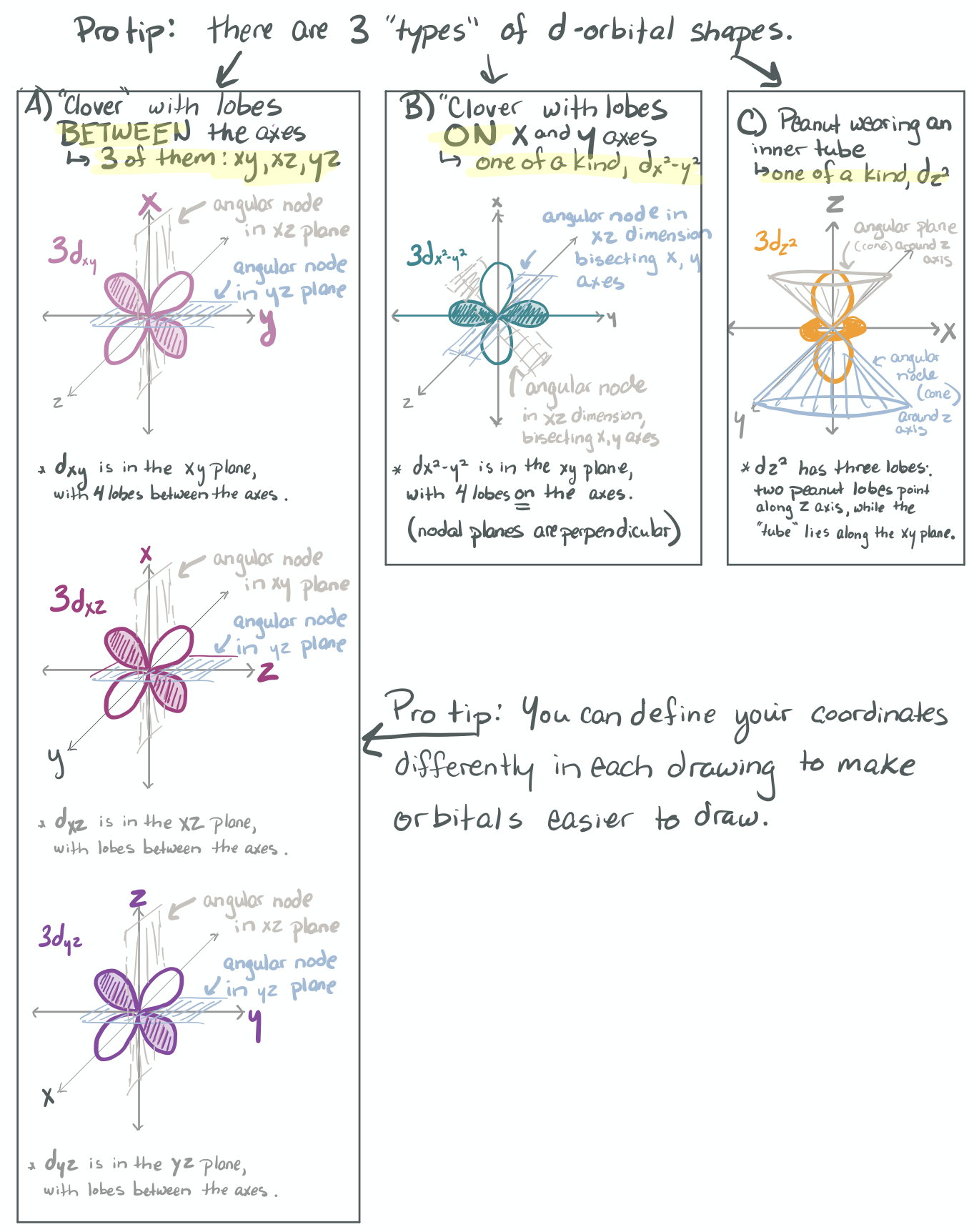
General shapes of common orbitals

The Schrödinger equation is a mathematical function in three-dimensional space. When a set of quantum numbers is applied (as variables) in the Schrödinger equation, the result (specifically, a three dimensional plot of the resulting function) is an atomic orbital: its three-dimensional "shape" and its energy. You should become very familiar with the general shapes and symmetry of the orbitals to succeed in this course; these shapes are shown in Table \(\PageIndex{2}\).

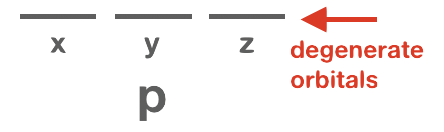
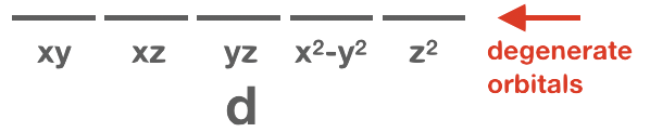
Orbitals that have the same or identical energy levels are referred to as degenerate. An example is the set of three orbitals within the 2p subshell: the 2p_x orbital has the same energy level as 2p_yand 2p_z.

Table \(\PageIndex{2}\). Quantum numbers and shapes of orbitals that you will see in this course.
SUBSHELL	s subshell	p subshell	d subshell
Value of \(l\)	ℓ = 0	ℓ = 1	ℓ = 2
Value(s) of \(m_l\)	m_ℓ = 0	m_ℓ= -1, 0, +1	m_ℓ= -2, -1, 0, +1, +2
Number of orbitals in this subshell:	One s orbital	Three p orbitals	Five d orbitals
General shape
How these are represented in electron orbital diagrams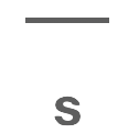

The shapes of orbitals are limited by boundary surfaces and nodes. The boundary surfaces define the surface of the orbital, while nodes separate different lobes. Please take notice not only of the general orbitals shapes shown above, but also of the shading/color of each lobe. The shading indicates the sign of the wavefunction in each lobe, and it is an important part of the orbital's symmetry. "Knowing" the shapes of these orbitals includes "knowing" the correct shading of each lobe.

Nodes (Angular and Radial)

The orbital shape represents the region in space where the electron is most likely to be found. The different lobes of an orbital are separated by regions in space where the probability of finding an electron is zero. These are nodes, and there are two types: angular nodes (planar nodes) and radial nodes (spherical nodes).

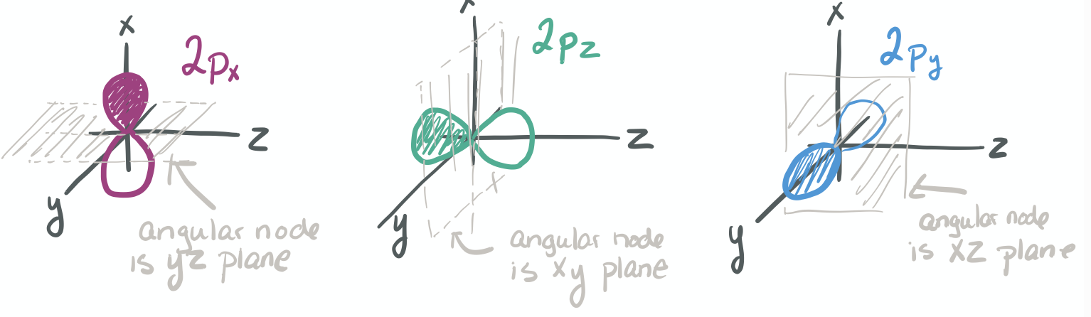
Angular Nodes

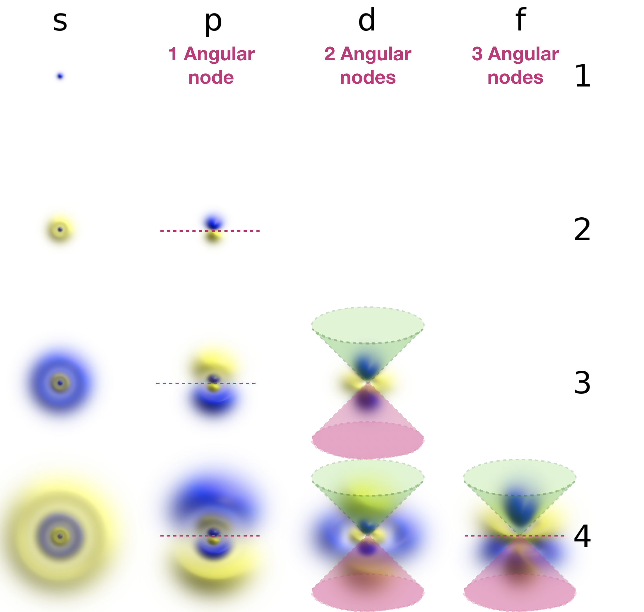
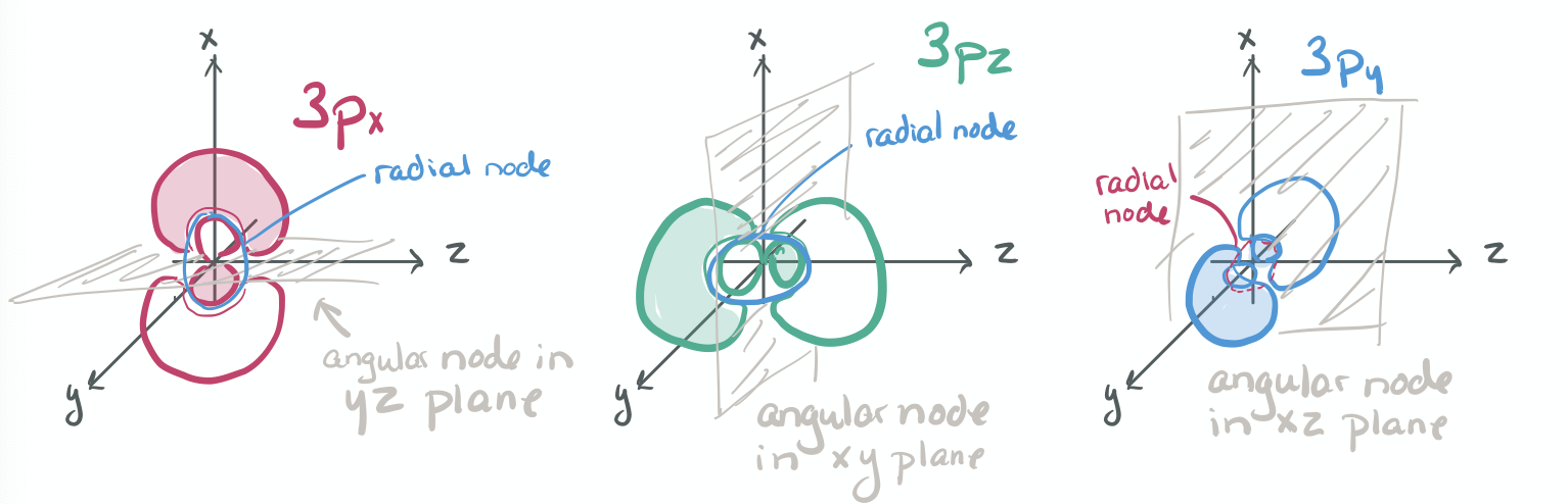
Angular nodes are planar in shape, and they depend upon the value of \(l\). The number of angular nodes in any orbital is equal to \(l\). This means that s-orbitals (\(l=0\)) have zero angular nodes, p-orbitals (\(l=1\)) have one angular node, d-orbitals (\(l=2\)) have two angular nodes, and so on. Planar nodes can be flat planes (like the nodes in all p orbitals) or they can have a conical shape, like the two angular nodes in the \(d_{Z^2}\) orbital. Angular nodes in some p and d orbitals are shown in Figure \(\PageIndex{2}\).

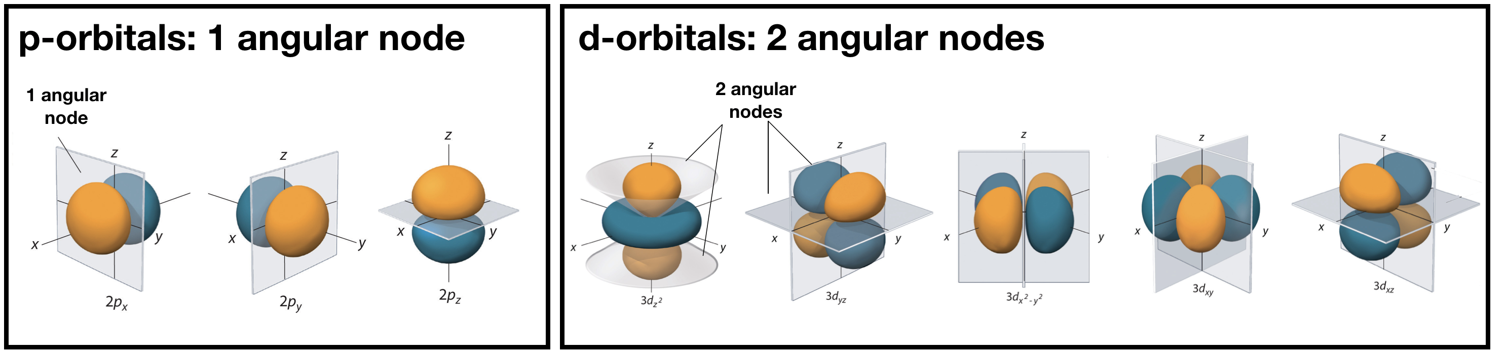
Screen Shot 2019-08-29 at 4.56.53 PM.png

Figure \(\PageIndex{2}\). The angular nodes in p-orbitals and d-orbitals are shown. Every p orbital has one angular node, and every d orbital has two angular nodes. The number of angular nodes in any orbital is equal to the value of the quantum number, \(l\).

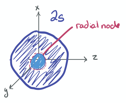
Radial Nodes

Radial nodes are spherical in shape and depend on the energy level and subshell (the values of \(n\) and \(l\)). The number of radial nodes is \(n-l-1\). Cut-a ways of the 1s, 2s, and 3s orbitals are shown in Figure \(\PageIndex{2}\) to illustrate radial nodes. An example of a radial node is the single node that occurs in the \(2s\) orbital (\(2-0-1=1\) node). In contrast, the 1s orbital has zero radial nodes (\(1-0-1=0\) nodes). Where there is a node, there is zero probability of finding an electron. In other words, electrons can't exist within a node.

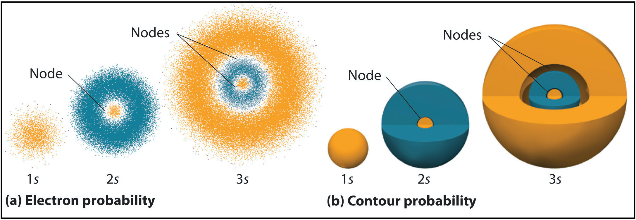
Figure \(\PageIndex{2}\). Visualization of the 1s, 2s, and 3s atomic orbitals. Each orbital is shown as both an electron probability density plot and a contour plot with labeled nodes.

Exercise \(\PageIndex{1}\): Identify Nodes

Inspect the figure/table below and identify as many planar nodes and radial nodes as you can. Make sure your answer matches the expected number of nodes that you would calculate based on the values of \(n\) and \(l\). The subshell type is listed along the top of the figure and the shell number (\(n\)) is listed along the right-hand side.

Figure \(\PageIndex{3}\). 3D views of some hydrogen-like atomic orbitals showing probability density and phase. (g orbitals and higher orbitals are not shown). From Wikipedia article on atomic orbitals. Attribution Geek3, Atomic-orbital-clouds spdf m0, CC BY-SA 4.0.

Hint

The number of nodes that you should expect for each orbital is:

Angular Nodes = \(l\), and the value of \(l\) correspond to the subshell type. An s orbital has \(l=0\), a p orbital has \(l=1\), a d orbital has \(l=2\), an f orbital has \(l=3\). Angular nodes are planar in shape.

Radial Nodes = \(n-l-1\). The values of \(n\) for each orbital are listed on the right-hand side. Radial nodes are spherical in shape.

Answer

The nodes are summarized in textual and visual form below:

1s: 0 angular nodes, 0 radial nodes

2s: 0 angular nodes, 1 radial nodes 2p: 1 angular nodes, 0 radial nodes

3s: 0 angular nodes, 2 radial nodes 3p: 1 angular nodes, 1 radial nodes 3d: 2 angular nodes, 0 radial nodes

4s: 0 angular nodes, 3 radial nodes 4p: 1 angular nodes, 2 radial nodes 4d: 2 angular nodes, 1 radial nodes 4f: 3 angular nodes, 0 radial nodes

Angular (planar) nodes are indicated as lines or cones in the annotated figure below:

Screen Shot 2019-11-11 at 4.10.12 PM.png

Radial (spherical) nodes are indicated on the annotated figure below:

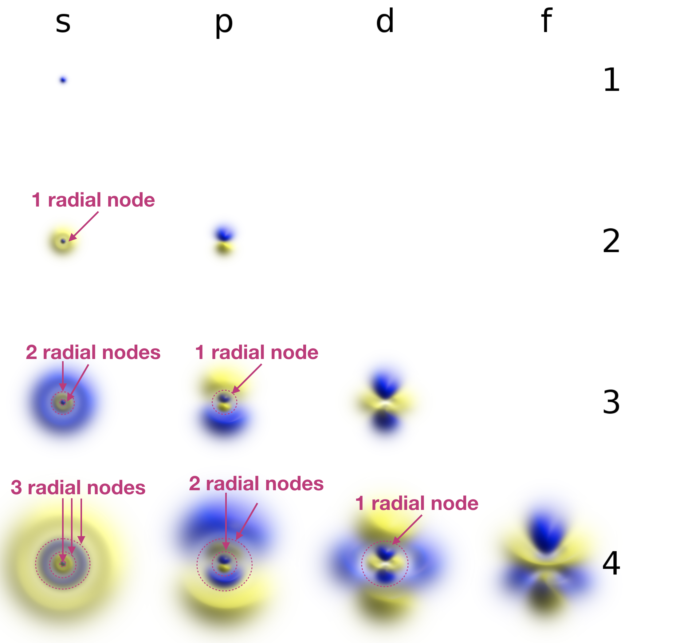
Screen Shot 2019-11-11 at 4.06.11 PM.png

The figures were harvested from the Wikipedia article on atomic orbitals. Geek3, Atomic-orbital-clouds spdf m0, nodes were labeled by Kathryn Haas, CC BY-SA 4.0.

Exercise \(\PageIndex{2}\): Identify direction of lobes and nodes

The ability to "know" your orbitals in the context of the Cartesian coordinate system is an important skill that will help you in this course. Please draw the shapes of all of the orbitals in the first three shells. For this problem, sketch the nodes and identify the plane in which the angular node(s) exist.

Practice the following habits now and throughout this course...

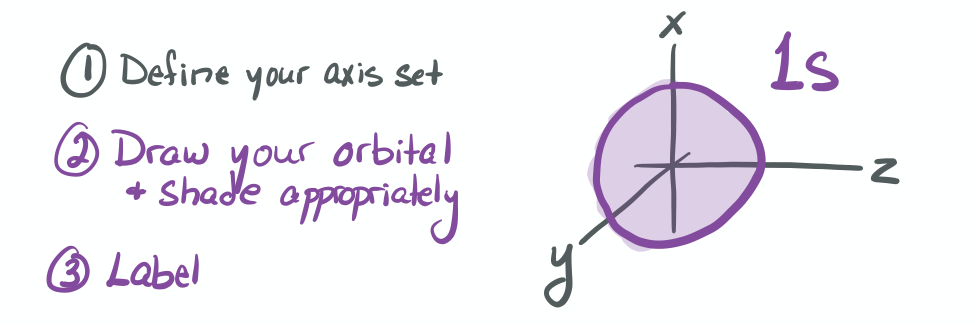
1) Draw each orbital superimposed on a labeled coordinate system (i.e. draw the x, y, z axes first and then draw your orbital on top of the axis set).

2) Always shade your orbitals appropriately to represent the signs of the wave function. (Color choice and shading of (+) vs (-) wave function is arbitrary)

3) Label your orbital clearly.

AnswerS

1s


2s


2p

3s

3p

3d

Contributions

Curated or created by Kathryn Haas