5.3: Determining the Sensitivity

To standardize an analytical method we also must determine the analyte’s sensitivity, k_A, in Equation 5.3.1 or Equation 5.3.2 .

\[S_{total} = k_A n_A + S_{reag} \label{5.1}\]

\[S_{total} = k_A C_A + S_{reag} \label{5.2}\]

In principle, it is possible to derive the value of k_A for any analytical method if we understand fully all the chemical reactions and physical processes responsible for the signal. Unfortunately, such calculations are not feasible if we lack a sufficiently developed theoretical model of the physical processes or if the chemical reaction’s evince non-ideal behavior. In such situations we must determine the value of k_A by analyzing one or more standard solutions, each of which contains a known amount of analyte. In this section we consider several approaches for determining the value of k_A. For simplicity we assume that S_reag is accounted for by a proper reagent blank, allowing us to replace S_total in Equation \ref{5.1} and Equation \ref{5.2} with the analyte’s signal, S_A.

\[S_A = k_A n_A \label{5.3}\]

\[S_A = k_A C_A \label{5.4}\]

Equation \ref{5.3} and Equation \ref{5.4} essentially are identical, differing only in whether we choose to express the amount of analyte in moles or as a concentration. For the remainder of this chapter we will limit our treatment to Equation \ref{5.4}. You can extend this treatment to Equation \ref{5.3} by replacing C_A with n_A.

Single-Point versus Multiple-Point Standardizations

The simplest way to determine the value of k_A in Equation \ref{5.4} is to use a single-point standardization in which we measure the signal for a standard, S_std, that contains a known concentration of analyte, C_std. Substituting these values into Equation \ref{5.4}

\[k_A = \frac {S_{std}} {C_{std}} \label{5.5}\]

gives us the value for k_A. Having determined k_A, we can calculate the concentration of analyte in a sample by measuring its signal, S_samp, and calculating C_A using Equation \ref{5.6}.

\[C_A = \frac {S_{samp}} {k_A} \label{5.6}\]

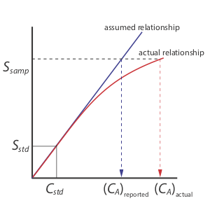
A single-point standardization is the least desirable method for standardizing a method. There are two reasons for this. First, any error in our determination of k_A carries over into our calculation of C_A. Second, our experimental value for k_A is based on a single concentration of analyte. To extend this value of k_A to other concentrations of analyte requires that we assume a linear relationship between the signal and the analyte’s concentration, an assumption that often is not true [Cardone, M. J.; Palmero, P. J.; Sybrandt, L. B. Anal. Chem. 1980, 52, 1187–1191]. Figure 5.3.1 shows how assuming a constant value of k_A leads to a determinate error in C_A if k_A becomes smaller at higher concentrations of analyte. Despite these limitations, single-point standardizations find routine use when the expected range for the analyte’s concentrations is small. Under these conditions it often is safe to assume that k_A is constant (although you should verify this assumption experimentally). This is the case, for example, in clinical labs where many automated analyzers use only a single standard.

Figure 5.3.1 : Example showing how a single-point standardization leads to a determinate error in an analyte’s reported concentration if we incorrectly assume that k_A is constant. The assumed relationship between S_samp and C_A is based on a single standard and is a straight-line; the actual relationship between S_samp and C_A becomes curved for larger concentrations of analyte.

The better way to standardize a method is to prepare a series of standards, each of which contains a different concentration of analyte. Standards are chosen such that they bracket the expected range for the analyte’s concentration. A multiple-point standardization should include at least three standards, although more are preferable. A plot of S_std versus C_std is called a calibration curve. The exact standardization, or calibration relationship, is determined by an appropriate curve-fitting algorithm.

Linear regression, which also is known as the method of least squares, is one such algorithm. Its use is covered in Section 5.4.

There are two advantages to a multiple-point standardization. First, although a determinate error in one standard introduces a determinate error, its effect is minimized by the remaining standards. Second, because we measure the signal for several concentrations of analyte, we no longer must assume k_A is independent of the analyte’s concentration. Instead, we can construct a calibration curve similar to the “actual relationship” in Figure 5.3.1 .

External Standards

The most common method of standardization uses one or more external standards, each of which contains a known concentration of analyte. We call these standards “external” because they are prepared and analyzed separate from the samples.

Appending the adjective “external” to the noun “standard” might strike you as odd at this point, as it seems reasonable to assume that standards and samples are analyzed separately. As we will soon learn, however, we can add standards to our samples and analyze both simultaneously.

Single External Standard

With a single external standard we determine k_A using EEquation \ref{5.5} and then calculate the concentration of analyte, C_A, using Equation \ref{5.6}.

Example 5.3.1

A spectrophotometric method for the quantitative analysis of Pb²⁺ in blood yields an S_std of 0.474 for a single standard for which the concentration of lead is 1.75 ppb. What is the concentration of Pb²⁺ in a sample of blood for which S_samp is 0.361?

Solution

Equation \ref{5.5} allows us to calculate the value of k_A using the data for the single external standard.

\[k_A = \frac {S_{std}} {C_{std}} = \frac {0.474} {1.75 \text{ ppb}} = 0.2709 \text{ ppb}^{-1} \nonumber\]

Having determined the value of k_A, we calculate the concentration of Pb²⁺ in the sample of blood is calculated using Equation \ref{5.6}.

\[C_A = \frac {S_{samp}} {k_A} = \frac {0.361} {0.2709 \text{ ppb}^{-1}} = 1.33 \text{ ppb} \nonumber\]

Multiple External Standards

Figure 5.3.2 shows a typical multiple-point external standardization. The volumetric flask on the left contains a reagent blank and the remaining volumetric flasks contain increasing concentrations of Cu²⁺. Shown below the volumetric flasks is the resulting calibration curve. Because this is the most common method of standardization, the resulting relationship is called a normal calibration curve.

Figure 5.3.2 : The photo at the top of the figure shows a reagent blank (far left) and a set of five external standards for Cu²⁺ with concentrations that increase from left-to-right. Shown below the external standards is the resulting normal calibration curve. The absorbance of each standard, S_std, is shown by the filled circles.

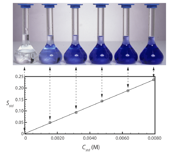
When a calibration curve is a straight-line, as it is in Figure 5.3.2 , the slope of the line gives the value of k_A. This is the most desirable situation because the method’s sensitivity remains constant throughout the analyte’s concentration range. When the calibration curve is not a straight-line, the method’s sensitivity is a function of the analyte’s concentration. In Figure 5.3.1 , for example, the value of k_A is greatest when the analyte’s concentration is small and it decreases continuously for higher concentrations of analyte. The value of k_A at any point along the calibration curve in Figure 5.3.1 is the slope at that point. In either case, a calibration curve allows to relate S_samp to the analyte’s concentration.

Example 5.3.2

A second spectrophotometric method for the quantitative analysis of Pb²⁺ in blood has a normal calibration curve for which

\[S_{std} = (0.296 \text{ ppb}^{-1} \times C_{std}) + 0.003 \nonumber\]

What is the concentration of Pb²⁺ in a sample of blood if S_samp is 0.397?

Solution

To determine the concentration of Pb²⁺ in the sample of blood, we replace S_std in the calibration equation with S_samp and solve for C_A.

\[C_A = \frac {S_{samp} - 0.003} {0.296 \text{ ppb}^{-1}} = \frac {0.397 - 0.003} {0.296 \text{ ppb}^{-1}} = 1.33 \text{ ppb} \nonumber\]

It is worth noting that the calibration equation in this problem includes an extra term that does not appear in Equation \ref{5.6}. Ideally we expect our calibration curve to have a signal of zero when C_A is zero. This is the purpose of using a reagent blank to correct the measured signal. The extra term of +0.003 in our calibration equation results from the uncertainty in measuring the signal for the reagent blank and the standards.

Exercise 5.3.1

Figure 5.3.2 shows a normal calibration curve for the quantitative analysis of Cu²⁺. The equation for the calibration curve is

\[S_{std} = 29.59 \text{ M}^{-1} \times C_{std} + 0.015 \nonumber\]

What is the concentration of Cu²⁺ in a sample whose absorbance, S_samp, is 0.114? Compare your answer to a one-point standardization where a standard of \(3.16 \times 10^{-3} \text{ M}\) Cu²⁺ gives a signal of 0.0931.

Answer

Substituting the sample’s absorbance into the calibration equation and solving for C_A give

\[S_{samp} = 0.114 = 29.59 \text{ M}^{-1} \times C_{A} + 0.015 \nonumber\]

\[C_A = 3.35 \times 10^{-3} \text{ M} \nonumber\]

For the one-point standardization, we first solve for k_A

\[k_A = \frac {S_{std}} {C_{std}} = \frac {0.0931} {3.16 \times 10^{-3} \text{ M}} = 29.46 \text{ M}^{-1} \nonumber\]

and then use this value of k_A to solve for C_A.

\[C_A = \frac {S_{samp}} {k_A} = \frac {0.114} {29.46 \text{ M}^{-1}} = 3.87 \times 10^{-3} \text{ M} \nonumber\]

When using multiple standards, the indeterminate errors that affect the signal for one standard are partially compensated for by the indeterminate errors that affect the other standards. The standard selected for the one-point standardization has a signal that is smaller than that predicted by the regression equation, which underestimates k_A and overestimates C_A.

An external standardization allows us to analyze a series of samples using a single calibration curve. This is an important advantage when we have many samples to analyze. Not surprisingly, many of the most common quantitative analytical methods use an external standardization.

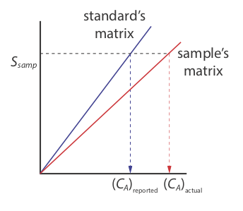
There is a serious limitation, however, to an external standardization. When we determine the value of k_A using Equation \ref{5.5}, the analyte is present in the external standard’s matrix, which usually is a much simpler matrix than that of our samples. When we use an external standardization we assume the matrix does not affect the value of k_A. If this is not true, then we introduce a proportional determinate error into our analysis. This is not the case in Figure 5.3.3 , for instance, where we show calibration curves for an analyte in the sample’s matrix and in the standard’s matrix. In this case, using the calibration curve for the external standards leads to a negative determinate error in analyte’s reported concentration. If we expect that matrix effects are important, then we try to match the standard’s matrix to that of the sample, a process known as matrix matching. If we are unsure of the sample’s matrix, then we must show that matrix effects are negligible or use an alternative method of standardization. Both approaches are discussed in the following section.

The matrix for the external standards in Figure 5.3.2 , for example, is dilute ammonia. Because the \(\ce{Cu(NH3)4^{2+}}\) complex absorbs more strongly than Cu²⁺, adding ammonia increases the signal’s magnitude. If we fail to add the same amount of ammonia to our samples, then we will introduce a proportional determinate error into our analysis.

Figure 5.3.3 : Calibration curves for an analyte in the standard’s matrix and in the sample’s matrix. If the matrix affects the value of k_A, as is the case here, then we introduce a proportional determinate error into our analysis if we use a normal calibration curve.

Standard Additions

We can avoid the complication of matching the matrix of the standards to the matrix of the sample if we carry out the standardization in the sample. This is known as the method of standard additions.

Single Standard Addition

The simplest version of a standard addition is shown in Figure 5.3.4 . First we add a portion of the sample, V_o, to a volumetric flask, dilute it to volume, V_f, and measure its signal, S_samp. Next, we add a second identical portion of sample to an equivalent volumetric flask along with a spike, V_std, of an external standard whose concentration is C_std. After we dilute the spiked sample to the same final volume, we measure its signal, S_spike.

Figure 5.3.4 : Illustration showing the method of standard additions. The volumetric flask on the left contains a portion of the sample, V_o, and the volumetric flask on the right contains an identical portion of the sample and a spike, V_std, of a standard solution of the analyte. Both flasks are diluted to the same final volume, V_f. The concentration of analyte in each flask is shown at the bottom of the figure where C_A is the analyte’s concentration in the original sample and C_std is the concentration of analyte in the external standard.

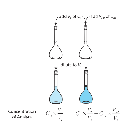
The following two equations relate S_samp and S_spike to the concentration of analyte, C_A, in the original sample.

\[S_{samp} = k_A C_A \frac {V_o} {V_f} \label{5.7}\]

\[S_{spike} = k_A \left( C_A \frac {V_o} {V_f} + C_{std} \frac {V_{std}} {V_f} \right) \label{5.8}\]

As long as V_std is small relative to V_o, the effect of the standard’s matrix on the sample’s matrix is insignificant. Under these conditions the value of k_A is the same in Equation \ref{5.7} and Equation \ref{5.8}. Solving both equations for k_A and equating gives

\[\frac {S_{samp}} {C_A \frac {V_o} {V_f}} = \frac {S_{spike}} {C_A \frac {V_o} {V_f} + C_{std} \frac {V_{std}} {V_f}} \label{5.9}\]

which we can solve for the concentration of analyte, C_A, in the original sample.

Example 5.3.3

A third spectrophotometric method for the quantitative analysis of Pb²⁺ in blood yields an S_samp of 0.193 when a 1.00 mL sample of blood is diluted to 5.00 mL. A second 1.00 mL sample of blood is spiked with 1.00 mL of a 1560-ppb Pb²⁺ external standard and diluted to 5.00 mL, yielding an S_spike of 0.419. What is the concentration of Pb²⁺ in the original sample of blood?

Solution

We begin by making appropriate substitutions into Equation \ref{5.9} and solving for C_A. Note that all volumes must be in the same units; thus, we first convert V_std from 1.00 mL to \(1.00 \times 10^{-3} \text{ mL}\).

\[\frac {0.193} {C_A \frac {1.00 \text{ mL}} {5.00 \text{ mL}}} = \frac {0.419} {C_A \frac {1.00 \text{ mL}} {5.00 \text{ mL}} + 1560 \text{ ppb} \frac {1.00 \times 10^{-3} \text{ mL}} {5.00 \text{ mL}}} \nonumber\]

\[\frac {0.193} {0.200C_A} = \frac {0.419} {0.200C_A + 0.3120 \text{ ppb}} \nonumber\]

\[0.0386C_A + 0.0602 \text{ ppb} = 0.0838 C_A \nonumber\]

\[0.0452 C_A = 0.0602 \text{ ppb} \nonumber\]

\[C_A = 1.33 \text{ ppb} \nonumber\]

The concentration of Pb²⁺ in the original sample of blood is 1.33 ppb.

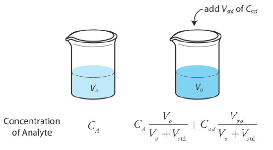
It also is possible to add the standard addition directly to the sample, measuring the signal both before and after the spike (Figure 5.3.5 ). In this case the final volume after the standard addition is V_o + V_std and Equation \ref{5.7}, Equation \ref{5.8}, and Equation \ref{5.9} become

\[S_{samp} = k_A C_A \nonumber\]

\[S_{spike} = k_A \left( C_A \frac {V_o} {V_o + V_{std}} + C_{std} \frac {V_{std}} {V_o + V_{std}} \right) \label{5.10}\]

\[\frac {S_{samp}} {C_A} = \frac {S_{spike}} {C_A \frac {V_o} {V_o + V_{std}} + C_{std} \frac {V_{std}} {V_o + V_{std}}} \label{5.11}\]

Figure 5.3.5 : Illustration showing an alternative form of the method of standard additions. In this case we add the spike of external standard directly to the sample without any further adjust in the volume.

Example 5.3.4

A fourth spectrophotometric method for the quantitative analysis of Pb²⁺ in blood yields an S_samp of 0.712 for a 5.00 mL sample of blood. After spiking the blood sample with 5.00 mL of a 1560-ppb Pb²⁺ external standard, an S_spike of 1.546 is measured. What is the concentration of Pb²⁺ in the original sample of blood?

Solution

\[\frac {0.712} {C_A} = \frac {1.546} {C_A \frac {5.00 \text{ mL}} {5.005 \text{ mL}} + 1560 \text{ ppb} \frac {5.00 \times 10^{-3} \text{ mL}} {5.005 \text{ mL}}} \nonumber\]

\[\frac {0.712} {C_A} = \frac {1.546} {0.9990C_A + 1.558 \text{ ppb}} \nonumber\]

\[0.7113C_A + 1.109 \text{ ppb} = 1.546C_A \nonumber\]

\[C_A = 1.33 \text{ ppb} \nonumber\]

The concentration of Pb²⁺ in the original sample of blood is 1.33 ppb.

Multiple Standard Additions

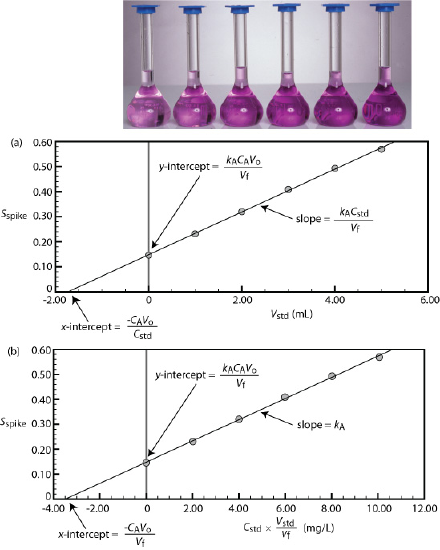
We can adapt a single-point standard addition into a multiple-point standard addition by preparing a series of samples that contain increasing amounts of the external standard. Figure 5.3.6 shows two ways to plot a standard addition calibration curve based on Equation \ref{5.8}. In Figure 5.3.6 a we plot S_spike against the volume of the spikes, V_std. If k_A is constant, then the calibration curve is a straight-line. It is easy to show that the x-intercept is equivalent to –C_AV_o/C_std.

Figure 5.3.6 : Shown at the top of the figure is a set of six standard additions for the determination of Mn²⁺. The flask on the left is a 25.00 mL sample diluted to 50.00 mL with water. The remaining flasks contain 25.00 mL of sample and, from left-to-right, 1.00, 2.00, 3.00, 4.00, and 5.00 mL spikes of an external standard that is 100.6 mg/L Mn²⁺. Shown below are two ways to plot the standard additions calibration curve. The absorbance for each standard addition, S_spike, is shown by the filled circles.

Example 5.3.5

Beginning with Equation \ref{5.8} show that the equations in Figure 5.3.6 a for the slope, the y-intercept, and the x-intercept are correct.

Solution

We begin by rewriting Equation \ref{5.8} as

\[S_{spike} = \frac {k_A C_A V_o} {V_f} + \frac {k_A C_{std}} {V_f} \times V_{std} \nonumber\]

which is in the form of the equation for a straight-line

\[y = y\text{-intercept} + \text{slope} \times x\text{-intercept} \nonumber\]

where y is S_spike and x is V_std. The slope of the line, therefore, is k_AC_std/V_f and the y-intercept is k_AC_AV_o/V_f. The x-intercept is the value of x when y is zero, or

\[0 = \frac {k_A C_A V_o} {V_f} + \frac {k_A C_{std}} {V_f} \times x\text{-intercept} \nonumber\]

\[x\text{-intercept} = - \frac {k_A C_A V_o / V_f} {K_A C_{std} / V_f} = - \frac {C_A V_o} {C_{std}} \nonumber\]

Exercise 5.3.2

Beginning with Equation \ref{5.8} show that the Equations in Figure 5.3.6 b for the slope, the y-intercept, and the x-intercept are correct.

Answer

We begin with Equation \ref{5.8}

\[S_{spike} = k_A \left( C_A \frac {V_o} {V_f} + C_{std} \frac {V_{std}} {V_f} \right) \nonumber\]

rewriting it as

\[S_{spike} = \frac {k_A C_A V_o} {V_f} + k_A \left( C_{std} \frac {V_{std}} {V_f} \right) \nonumber\]

which is in the form of the linear equation

\[y = y\text{-intercept} + \text{slope} \times x\text{-intercept} \nonumber\]

where y is S_spike and x is C_std \(\times\) V_std/V_f. The slope of the line, therefore, is k_A, and the y-intercept is k_AC_AV_o/V_f. The x-intercept is the value of x when y is zero, or

\[x\text{-intercept} = - \frac {k_A C_A V_o/V_F} {k_A} = - \frac {C_A V_o} {V_f} \nonumber\]

Because we know the volume of the original sample, V_o, and the concentration of the external standard, C_std, we can calculate the analyte’s concentrations from the x-intercept of a multiple-point standard additions.

Example 5.3.6

A fifth spectrophotometric method for the quantitative analysis of Pb²⁺ in blood uses a multiple-point standard addition based on Equation \ref{5.8}. The original blood sample has a volume of 1.00 mL and the standard used for spiking the sample has a concentration of 1560 ppb Pb²⁺. All samples were diluted to 5.00 mL before measuring the signal. A calibration curve of S_spike versus V_std has the following equation

\[S_{spike} = 0.266 + 312 \text{ mL}^{-1} \times V_{std} \nonumber\]

What is the concentration of Pb²⁺ in the original sample of blood?

Solution

To find the x-intercept we set S_spike equal to zero.

\[S_{spike} = 0.266 + 312 \text{ mL}^{-1} \times V_{std} \nonumber\]

Solving for V_std, we obtain a value of \(-8.526 \times 10^{-4} \text{ mL}\) for the x-intercept. Substituting the x-intercept’s value into the equation from Figure 5.3.6 a

\[-8.526 \times 10^{-4} \text{ mL} = - \frac {C_A V_o} {C_{std}} = - \frac {C_A \times 1.00 \text{ mL}} {1560 \text{ ppb}} \nonumber\]

and solving for C_A gives the concentration of Pb²⁺ in the blood sample as 1.33 ppb.

Exercise 5.3.3

Figure 5.3.6 shows a standard additions calibration curve for the quantitative analysis of Mn²⁺. Each solution contains 25.00 mL of the original sample and either 0, 1.00, 2.00, 3.00, 4.00, or 5.00 mL of a 100.6 mg/L external standard of Mn²⁺. All standard addition samples were diluted to 50.00 mL with water before reading the absorbance. The equation for the calibration curve in Figure 5.3.6 a is

\[S_{std} = 0.0854 \times V_{std} + 0.1478 \nonumber\]

What is the concentration of Mn²⁺ in this sample? Compare your answer to the data in Figure 5.3.6 b, for which the calibration curve is

\[S_{std} = 0.425 \times C_{std}(V_{std}/V_f) + 0.1478 \nonumber\]

Answer

Using the calibration equation from Figure 5.3.6 a, we find that the x-intercept is

\[x\text{-intercept} = - \frac {0.1478} {0.0854 \text{ mL}^{-1}} = - 1.731 \text{ mL} \nonumber\]

If we plug this result into the equation for the x-intercept and solve for C_A, we find that the concentration of Mn²⁺ is

\[C_A = - \frac {x\text{-intercept} \times C_{std}} {V_o} = - \frac {-1.731 \text{ mL} \times 100.6 \text{ mg/L}} {25.00 \text{ mL}} = 6.96 \text{ mg/L} \nonumber\]

For Figure 5.3.6 b, the x-intercept is

\[x\text{-intercept} = - \frac {0.1478} {0.0425 \text{ mL/mg}} = - 3.478 \text{ mg/mL} \nonumber\]

and the concentration of Mn²⁺ is

\[C_A = - \frac {x\text{-intercept} \times V_f} {V_o} = - \frac {-3.478 \text{ mg/mL} \times 50.00 \text{ mL}} {25.00 \text{ mL}} = 6.96 \text{ mg/L} \nonumber\]

Since we construct a standard additions calibration curve in the sample, we can not use the calibration equation for other samples. Each sample, therefore, requires its own standard additions calibration curve. This is a serious drawback if you have many samples. For example, suppose you need to analyze 10 samples using a five-point calibration curve. For a normal calibration curve you need to analyze only 15 solutions (five standards and ten samples). If you use the method of standard additions, however, you must analyze 50 solutions (each of the ten samples is analyzed five times, once before spiking and after each of four spikes).

Using a Standard Addition to Identify Matrix Effects

We can use the method of standard additions to validate an external standardization when matrix matching is not feasible. First, we prepare a normal calibration curve of S_std versus C_std and determine the value of k_A from its slope. Next, we prepare a standard additions calibration curve using Equation \ref{5.8}, plotting the data as shown in Figure 5.3.6 b. The slope of this standard additions calibration curve provides an independent determination of k_A. If there is no significant difference between the two values of k_A, then we can ignore the difference between the sample’s matrix and that of the external standards. When the values of k_A are significantly different, then using a normal calibration curve introduces a proportional determinate error.

Internal Standards

To use an external standardization or the method of standard additions, we must be able to treat identically all samples and standards. When this is not possible, the accuracy and precision of our standardization may suffer. For example, if our analyte is in a volatile solvent, then its concentration will increase if we lose solvent to evaporation. Suppose we have a sample and a standard with identical concentrations of analyte and identical signals. If both experience the same proportional loss of solvent, then their respective concentrations of analyte and signals remain identical. In effect, we can ignore evaporation if the samples and the standards experience an equivalent loss of solvent. If an identical standard and sample lose different amounts of solvent, however, then their respective concentrations and signals are no longer equal. In this case a simple external standardization or standard addition is not possible.

We can still complete a standardization if we reference the analyte’s signal to a signal from another species that we add to all samples and standards. The species, which we call an internal standard, must be different than the analyte.

Because the analyte and the internal standard receive the same treatment, the ratio of their signals is unaffected by any lack of reproducibility in the procedure. If a solution contains an analyte of concentration C_A and an internal standard of concentration C_IS, then the signals due to the analyte, S_A, and the internal standard, S_IS, are

\[S_A = k_A C_A \nonumber\]

\[S_{IS} = k_{SI} C_{IS} \nonumber\]

where \(k_A\) and \(k_{IS}\) are the sensitivities for the analyte and the internal standard, respectively. Taking the ratio of the two signals gives the fundamental equation for an internal standardization.

\[\frac {S_A} {S_{IS}} = \frac {k_A C_A} {k_{IS} C_{IS}} = K \times \frac {C_A} {C_{IS}} \label{5.12}\]

Because K is a ratio of the analyte’s sensitivity and the internal standard’s sensitivity, it is not necessary to determine independently values for either k_A or k_IS.

Single Internal Standard

In a single-point internal standardization, we prepare a single standard that contains the analyte and the internal standard, and use it to determine the value of K in Equation \ref{5.12}.

\[K = \left( \frac {C_{IS}} {C_A} \right)_{std} \times \left( \frac {S_A} {S_{IS}} \right)_{std} \label{5.13}\]

Having standardized the method, the analyte’s concentration is given by

\[C_A = \frac {C_{IS}} {K} \times \left( \frac {S_A} {S_{IS}} \right)_{samp} \nonumber\]

Example 5.3.7

A sixth spectrophotometric method for the quantitative analysis of Pb²⁺ in blood uses Cu²⁺ as an internal standard. A standard that is 1.75 ppb Pb²⁺ and 2.25 ppb Cu²⁺ yields a ratio of (S_A/S_IS)_std of 2.37. A sample of blood spiked with the same concentration of Cu²⁺ gives a signal ratio, (S_A/S_IS)_samp, of 1.80. What is the concentration of Pb²⁺ in the sample of blood?

Solution

Equation \ref{5.13} allows us to calculate the value of K using the data for the standard

\[K = \left( \frac {C_{IS}} {C_A} \right)_{std} \times \left( \frac {S_A} {S_{IS}} \right)_{std} = \frac {2.25 \text{ ppb } \ce{Cu^{2+}}} {1.75 \text{ ppb } \ce{Pb^{2+}}} \times 2.37 = 3.05 \frac {\text{ppb } \ce{Cu^{2+}}} {\text{ppb } \ce{Pb^{2+}}} \nonumber\]

The concentration of Pb²⁺, therefore, is

\[C_A = \frac {C_{IS}} {K} \times \left( \frac {S_A} {S_{IS}} \right)_{samp} = \frac {2.25 \text{ ppb } \ce{Cu^{2+}}} {3.05 \frac {\text{ppb } \ce{Cu^{2+}}} {\text{ppb } \ce{Pb^{2+}}}} \times 1.80 = 1.33 \text{ ppb } \ce{Pb^{2+}} \nonumber\]

Multiple Internal Standards

A single-point internal standardization has the same limitations as a single-point normal calibration. To construct an internal standard calibration curve we prepare a series of standards, each of which contains the same concentration of internal standard and a different concentrations of analyte. Under these conditions a calibration curve of (S_A/S_IS)_std versus C_A is linear with a slope of K/C_IS.

Although the usual practice is to prepare the standards so that each contains an identical amount of the internal standard, this is not a requirement.

Example 5.3.8

A seventh spectrophotometric method for the quantitative analysis of Pb²⁺ in blood gives a linear internal standards calibration curve for which

\[\left( \frac {S_A} {S_{IS}} \right)_{std} = (2.11 \text{ ppb}^{-1} \times C_A) - 0.006 \nonumber\]

What is the ppb Pb²⁺ in a sample of blood if (S_A/S_IS)samp is 2.80?

Solution

To determine the concentration of Pb²⁺ in the sample of blood we replace (S_A/S_IS)_std in the calibration equation with (S_A/S_IS)_samp and solve for C_A.

\[C_A = \frac {\left( \frac {S_A} {S_{IS}} \right)_{samp} + 0.006} {2.11 \text{ ppb}^{-1}} = \frac {2.80 + 0.006} {2.11 \text{ ppb}^{-1}} = 1.33 \text{ ppb } \ce{Pb^{2+}} \nonumber\]

The concentration of Pb²⁺ in the sample of blood is 1.33 ppb.

In some circumstances it is not possible to prepare the standards so that each contains the same concentration of internal standard. This is the case, for example, when we prepare samples by mass instead of volume. We can still prepare a calibration curve, however, by plotting \((S_A / S_{IS})_{std}\) versus C_A/C_IS, giving a linear calibration curve with a slope of K.

You might wonder if it is possible to include an internal standard in the method of standard additions to correct for both matrix effects and uncontrolled variations between samples; well, the answer is yes as described in the paper “Standard Dilution Analysis,” the full reference for which is Jones, W. B.; Donati, G. L.; Calloway, C. P.; Jones, B. T. Anal. Chem. 2015, 87, 2321-2327.