4.1: The Wavefunction Specifies the State of a System

In classical mechanics, the configuration or state of a system is given by a point \(( x , p )\) in the space of coordinates and momenta. This specifies everything else in the system in a fully deterministic way, in that any observable \(Q\) that can be expressed as \(Q ( x , p )\) can be found, and any that cannot is irrelevant. Yet, as we have seen with the diffraction of electrons, it is impossible to know both the position and momentum of the electron exactly at every point along the trajectory. This is mathematically expressed as the famous position-momentum uncertainty principle. Hence, specifying a state by \(( x , p )\) in classical mechanics clearly will not work in quantum mechanics. So what specifies the state of a quantum system? This is where the first Postulate of quantum mechanics comes in.

Postulate I

The state of the system is completely specified by \(\psi\). All possible information about the system can be found in the wavefunction \(\psi\).

The properties of a quantum mechanical system are determined by a wavefunction \(\psi(r,t)\) that depends upon the spatial coordinates of the system and time, \(r\) and \(t\). For a single particle system, \(r\) is the set of coordinates of that particle \(r = (x_1, y_1, z_1)\). For more than one particle, \(r\) is used to represent the complete set of coordinates \(r = (x_1, y_1, z_1, x_2, y_2, z_2,\dots x_n, y_n, z_n)\). Since the state of a system is defined by its properties, \(\psi\) specifies or identifies the state and sometimes is called the state function rather than the wavefunction.

What does \(\psi\) mean? This is best answered in terms of the probability density \(P(x)\) that determines the probability (density) that an object in the state \(ψ ( x )\) will be found at position \(x\) (the Born interpretation).

\[ \begin{align} P ( x ) &= ψ^*(x)ψ(x) \\[4pt] &= |ψ(x)| ^2 \label{norm} \end{align}\]

Hence, for valid (e.g., well-behaved) wavefunctions, the normalized probability in Equation \(\ref{norm}\) holds true, such that the integral over all space is equal to 1.

\[\int_{-\infty}^\infty \psi^*(x)\psi(x)\;dx=1 \label{4.1.1}\]

this means is that the chance to find a particle is 100% over all space.

Let us examine this set of examples in further detail in Figure \(\PageIndex{1}\). The first wavefunction \(ψ_1\) is sharply peaked at a particular value of \(x\), and the probability density, being its square, is likewise peaked there as well. This is the wavefunction for a particle well localized at a position given by the center of the peak, as the probability density is high there, and the width of the peak is small, so the uncertainty in the position is very small.

Figure \(\PageIndex{1}\): Examples of good wavefunctions, \(\psi(x)\), (red, top) and corresponding probability densities, \(P(x)\), (blue, bottom).

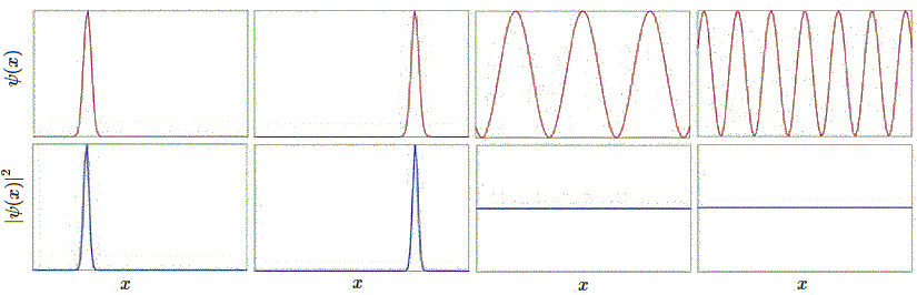
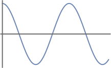
The second wavefunction \(ψ_2\) has the same peak profile, but shifted to a different position center. All of the properties of the first wavefunction hold here too, so this simply describes a particle that is well-localized at that different position. The third and fourth wavefunctions \(ψ_3\) and \(ψ_4\) respectively look like sinusoids of different spatial periods. The wavefunctions are actually complex of the form

\[ψ ( x ) = Ne^{ikx}\]

so only the real part is being plotted in Figure \(\PageIndex{1}\). Note that even though the periods, \(k\), of the oscillating wavefunctions are different,

\[ P(x) = ψ^*(x)ψ(x) = | e^{ikx} |^2 = N^2e^{-ikx} \times e^{ikx} = N^2 \]

for all \(k\), so the corresponding probability densities, \(P(x)\), are the same except for the nor­malization constant (Equation \(\ref{norm}\)). We saw before that it does not make a whole lot of sense to think of a sinusoidal wave as being localized in some place. Indeed, the positions for these two wavefunctions are ill-defined, so they are not well-localized, and the uncertainty in the position is large in each case. This is Heisenberg Uncertainty Principle in action.

Ill-behaved (invalid) Wavefunctions

The Born interpretation in Equation \(\ref{norm}\) means that many wavefunctions which would be acceptable mathematical solutions of the Schrödinger equation are not acceptable because of their implications for the physical properties of the system. To satisfy this interpretation, wavefunctions must be:

• single valued,
• continuous, and
• finite.

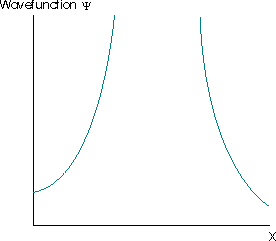
These aspects mean that the valid wavefunction must be one-to-one, it cannot have an undefined slope, and cannot go to \(-\infty\) or \(+\infty\). For example, the wavefunction must not be infinite over any finite region. If it is, then the integral in Equation \(\ref{4.1.1}\) is equal to infinity. This implies that the particle described by such a wavefunction has a zero probability of being anywhere where the wavefunction is not infinite, but is certain to be found at all points where the wavefunction is infinite.

Figure \(\PageIndex{2}\): A invalid wavefunction since the amplitude is going to infinity over a region (the middle in this case).

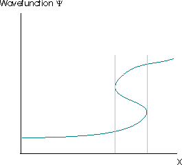
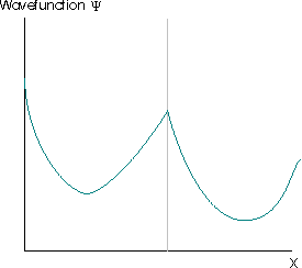
The Born interpretation also renders unacceptable solutions of the Schrödinger equation for which \(|ψ(x)|^2\) has more than one value at any point. This would suggest that there were multiple different probabilities of finding the particle at that point, which is clearly absurd. The requirement that the square modulus of the wavefunction must be single-valued usually implies that the wavefunction itself must be single valued. The wavefunction in Figure \(\PageIndex{3}\) violates this requirement. The grey lines indicate the region where the wavefunction is multivalued.

Figure \(\PageIndex{3}\): A invalid wavefunction since the wavefunction is not a function (i.e., not one-to-one).

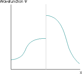
Further restrictions arise because the wavefunction must satisfy the Schrödinger equation, which is a second-order differential equation. This implies that the second derivative of the function must exist, which implies that the first derivative of the wavefunction to exist (otherwise the second derivative is also undefined and the wavefunction cannot be a solution of the Schrödinger equation). The wavefunctions in Figure \(\PageIndex{4}\) are also not acceptable for these reasons.

Figure \(\PageIndex{4}\): Invalid wavefunctions. (left) The first derivative of a function gives its gradient at a given point, and it thus exists as long as the function is continuous - only if there is a break in the function is there a point at which its first derivative does not exist. (right) The second derivative of this wavefunction is discontinuous at the point indicated, where the gradient of the line changes by more than 180º. In practice, this requirement may be somewhat flexible, particularly if the potential energy of the system shows rapid changes with distance.

Exercise \(\PageIndex{1}\)

Determine if each of the following functions is acceptable or not as a wavefunction over the indicated regions

1. \(\cos x \) over \((0,\infty)\)
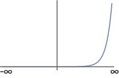
2. \(e^x \) over \((-\infty,\infty)\)
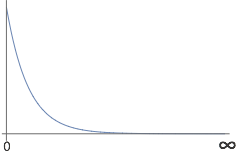
3. \(e^{-x} \) over \([0,\infty)\)
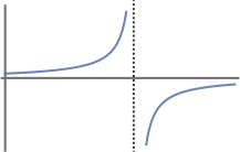
4. \(\tan \theta\) over \([0, 2\theta]\)

Solution a

This is not an acceptable wavefunction. It is single-valued across the entire range. There is only value for each value of x. It is continuous over the defined limits of integration, as we can see from a plot given below. However, it is not square-integrable. \(\int_{0}^{\infty} | \cos(x) |^2 dx \; \xcancel{<} \; \infty \)

Solution b

This is not an acceptable wavefunction. Over the limits of integration from \( -\infty \) to \( \infty \), this function is not square-integrable. Note in the plot below, how the function is indefinite approaching the limits of \( \infty \).

Solution c

This is an acceptable wavefunction over the given limits. It is finite over the given limits. It is continuous within given limits. It is single-valued. It is square-integrable \( \int_{0}^{\infty} | \Psi(x) |^2 dx = \frac{1}{2} \).

Solution d

This is not an acceptable wavefunction. It is discontinuous over the limits of integration.

Contributors

• Prof. Allan Adams, Prof. Matthew Evans, Prof. Barton Zwiebach (used with permission, MIT OpenCourseWare)