3.7: The Average Momentum of a Particle in a Box is Zero

Now that we have mathematical expressions for the wavefunctions and energies for the particle-in-a-box, we can answer a number of interesting questions. The answers to these questions use quantum mechanics to predict some important and general properties for electrons, atoms, molecules, gases, liquids, and solids. Key to addressing these questions is the formulation and use of expectation values. This is demonstrated below and used in the context of evaluating average properties (momentum of the particle in a box for the case below).

Expectation Values

The expectation value is the probabilistic expected value of the result (measurement) of an experiment. It is not the most probable value of a measurement; indeed the expectation value may have zero probability of occurring. The expected value (or expectation, mathematical expectation, mean, or first moment) refers to the value of a variable one would "expect" to find if one could repeat the random variable process an infinite number of times and take the average of the values obtained. More formally, the expected value is a weighted average of all possible values.

Example \(\PageIndex{1}\): Classical Expectation Value of Exam Scores (a discretized example)

A classical example is calculating the expectation value (i.e. average) of the exam grades in the class. For example if the class scores for an exam were

65

67

94

43

67

76

94

67

The discrete way is to sum up all scores and divide by the number of students:

\[\langle s \rangle = \dfrac{\sum_i^N s(i)}{N} \label{Cl1}\]

which of this example of scores is

\[ \begin{align*} \langle s \rangle &= \dfrac{65 + 67 +94 +43 +67+76+94+76}{8} \\[4pt] &= 71.625 \end{align*}\]

Notice that the average is not an allowable score on an individual exam. Equation \(\ref{Cl1}\) can be rewritten with "probability" or "probability weights"

\[\langle s \rangle = \sum_i^N s(i) P_s(i) \label{Cl2}\]

where \(P_s(i)\) is the probability of observing a score of \(s\). This is just the number of times it occurs in a dataset divided by the number of elements in that data set. Applying Equation \ref{Cl2} to the set of scores, we need to calculate these wights:

Score	65	67	94	43	76
\(P_s\)	1/8	3/8	2/8	1/8	1/8

As with all probabilities, the sum of all probabilities possible must be one. These confirm that for the weights here:

\[ \dfrac{1}{8} + \dfrac{3}{8} + \dfrac{2}{8} + \dfrac{1}{8} + \dfrac{1}{8} = \dfrac{8}{8} =1\]

This the discretized "normalization" criterion (the same as why we normalize wavefunctions.

So, now we can use Equation \(\ref{Cl2}\) properly

\[ \begin{align*} \langle s \rangle &= 65 \times \dfrac{1}{8} + 67\times \dfrac{3}{8} +94\times \dfrac{2}{8} + 43 \times\dfrac{1}{8} +76\times \dfrac{1}{8} \\[4pt] &= 71.625 \end{align*}\]

Hence, Equation \(\ref{Cl2}\) gives the same result, as expected, from Equation \(\ref{Cl1}\).

The extension of the classical expectation (average) approach in Example \(\PageIndex{1}\) using Equation \ref{Cl2} to evaluating quantum mechanical expectation values requires three small changes:

1. Switch from descretized to continuous variables
2. Substitute the wavefunction squared for the probability weights (i.e., the probability distribution)
3. Use an operator instead of the scalar

Hence, the quantum mechanical expectation value \(\langle o \rangle\) for an observable, \(o\), associated with an operator, \(\hat{O}\), is given by

\[ \langle o \rangle = \int _{-\infty}^{+\infty} \psi^* \hat{O} \psi \, dx \label{expect}\]

where \(x\) is the range of space that is integrated over (i.e., an integration over all possible probabilities). The expectation value changes as the wavefunction changes and the operator used (i.e, which observable you are averaging over).

In general, changing the wavefunction changes the expectation value for that operator for a state defined by that wavefunction.

Average Energy of a Particle in a Box

If we generalize this conclusion, such integrals give the average value for any physical quantity by using the operator corresponding to that physical observable in the integral in Equation \(\ref{expect}\). In the equation below, the symbol \(\left \langle H \right \rangle\) is used to denote the average value for the total energy.

\[ \begin{align} \left \langle H \right \rangle &= \int \limits ^{\infty}_{-\infty} \psi ^* (x) \hat {H} \psi (x) dx \\[4pt] &= \int \limits ^{\infty}_{-\infty} \psi ^* (x) \hat {KE} \psi (x) dx + \int \limits ^{\infty}_{-\infty} \psi ^* (x) \hat {V} \psi (x) dx \\[4pt] &= \underset{\text {average kinetic energy} }{ \int \limits ^{\infty}_{-\infty} \psi ^* (x) \left ( \frac {-\hbar ^2}{2m} \right ) \frac {\partial ^2 }{ \partial x^2} \psi (x) dx} + \underset{ \text {average potential energy} }{\int \limits ^{\infty}_{-\infty} \psi ^* (x) \hat{V} (x) \psi (x) dx} \label{3-35} \end{align}\]

The Hamiltonian operator consists of a kinetic energy term and a potential energy term. The kinetic energy operator involves differentiation of the wavefunction to the right of it. This step must be completed before multiplying by the complex conjugate of the wavefunction. The potential energy, however, usually depends only on position and not momentum (i.e., it involves conservative forces). The potential energy operator therefore only involves the coordinates of a particle and does not involve differentiation. For this reason we do not need to use a caret over \(V\) in Equation \(\ref{3-35}\).

Equation \ref{3-35} can be simplified

\[ \langle H \rangle = \langle KE \rangle + \langle V \rangle \label{3-35 braket}\]

The potential energy integral then involves only products of functions, and the order of multiplication does not affect the result, e.g. 6×4 = 4×6 = 24. This property is called the commutative property. The average potential energy therefore can be written as

\[ \left \langle V \right \rangle = \int \limits ^{\infty}_{-\infty} V (x) \psi ^* (x) \psi (x) dx \label{3-36}\]

This integral is telling us to take the probability that the particle is in the interval \(dx\) at \(x\), which is \(ψ^*(x)ψ(x)dx\), multiply this probability by the potential energy at \(x\), and sum (i.e., integrate) over all possible values of \(x\). This procedure is just the way to calculate the average potential energy \(\left \langle V \right \rangle\) of the particle.

Exercise \(\PageIndex{2}\): Particle in Box

Evaluate the two integrals in Equation \(\ref{3-35}\) for the PIB wavefunction \(ψ(x) = \sqrt{\dfrac{2}{L}} \sin(k x)\) with the potential function \(V(x) = 0\) from 0 to the length of a box \(L\) with \(k= \dfrac{\pi }{L}\).

Solution

The average kinetic energy is

\[\begin{align*} \langle KE \rangle &= \int \limits ^{L}_{0} \left(\sqrt{\dfrac{2}{L}}\right) \sin(kx) \left ( \frac {-\hbar ^2}{2m} \right ) \frac {\partial ^2 }{ \partial x^2} \left(\sqrt{\dfrac{2}{L}}\right) \sin(kx) dx \\[4pt] &= \left(\dfrac{2}{L}\right) \int \limits ^{L}_{0} \sin(kx) \left ( \frac {-\hbar ^2}{2m} \right ) \frac {\partial }{ \partial x} \cos(kx)(k) dx \\[4pt] &= \left(\dfrac{2}{L}\right) \int \limits ^{L}_{0} \sin(kx) \left ( \frac {-\hbar ^2}{2m} \right ) \sin(kx)(k)(-k) dx \\[4pt] &= \left(\dfrac{2}{L}\right) \left ( \frac { k^2 \hbar ^2}{2m} \right ) \int \limits ^{L}_{0} \sin^2(kx) dx \end{align*}\]

We can solve this intragral using the standard half-angle represention from an integral table. Or we can recognize that we already did this integral when we normalized the PIB wavefunction by rewriting this integral:

\[\begin{align*} \langle KE \rangle &= \left(\dfrac{2}{L}\right) \left ( \frac { k^2 \hbar ^2}{2m} \right ) \int \limits ^{L}_{0} \sin^2(kx) dx \\[4pt] &= \left ( \frac { k^2 \hbar ^2}{2m} \right ) \int \limits ^{L}_{0} \left(\dfrac{2}{L}\right) \sin^2(kx) dx \\[4pt] &=\left ( \frac { k^2 \hbar ^2}{2m} \right ) \cancelto{1}{\int \limits ^{L}_{0} \psi^*(x)\psi(x) dx} \\[4pt] &= \frac { k^2 \hbar ^2}{2m} \end{align*}\]

Thus, the average value for the total energy of this particular system is

\[ \langle KE \rangle = \dfrac { k^2 \hbar ^2}{2m} = \dfrac { \pi^2 \hbar ^2}{2mL^2} \nonumber\]

Hence, the average kinetic energy of the wavefunction is dependent on the \(n\) quantum number

The average potential energy is

\[ \langle V \rangle = \int \limits ^{\infty}_{-\infty} \sin(kx) 0 \sin(kx) dx = 0 \nonumber\]

Thus, the average potential energy of the PIB is 0 irrespective of the wavefunction.

Hence via Equation \ref{3-35 braket} for this system and set of wavefunctions

\[ \langle H \rangle = \dfrac { \pi^2 \hbar ^2}{2mL^2} \nonumber\]

This is the same result obtained from solving the eigenvalue equation for the PIB. However, if the wavefunctions used were NOT eigenstates of energy, then we cannot use the eigenvalue approach and need to rely on the expectation values to describe the energy of the system.

What is the lowest energy for a particle in a box? The lowest energy level is \(E_1\), and it is important to recognize that this lowest energy of a particle in a box is not zero. This finite energy is called the zero-point energy, and the motion associated with this energy is called the zero-point motion. Any system that is restricted to some region of space is said to be bound. The zero-point energy and motion are manifestations of the wave properties and the Heisenberg Uncertainty Principle, and are general properties of bound quantum mechanical systems.

Exercise \(\PageIndex{2}\): Progressing to the Classical Limit

What happens to the energy level spacing for a particle-in-a-box when \(mL^2\) becomes much larger than \(h^2\)? What does this result imply about the relevance of quantization of energy to baseballs in a box between the pitching mound and home plate? What implications does quantum mechanics have for the game of baseball in a world where \(h\) is so large that baseballs exhibit quantum effects?

Answer:

As \(mL^2\) becomes much larger than \(h^2\), as everyday objects are, the spacing between energy levels becomes much smaller. This shows how the quantizations of energy levels become irrelevant for an everyday object, as the quantizations of the energy of baseballs in a box between the pitching mound and home plate would appear particularly continuous for such a relatively large mass and box length. If h were so large that a baseball experiences quantum effects then a game of baseball would be far less predictable, in a classical world the position of a baseball can be easily predicted by the everyday understanding of projectile motion, however, in such a quantum world the baseball would not behave with expected projectile motion but instead behave wave-like with a probability of being in a certain position.

The first derivative of a function is the rate of change of the function, and the second derivative is the rate of change in the rate of change, also known as the curvature. A function with a large second derivative is changing very rapidly. Since the second derivative of the wavefunction occurs in the Hamiltonian operator that is used to calculate the energy by using the Schrödinger equation, a wavefunction that has sharper curvatures than another, i.e. larger second derivatives, should correspond to a state having a higher energy. A wavefunction with more nodes than another over the same region of space must have sharper curvatures and larger second derivatives, and therefore should correspond to a higher energy state.

Exercise \(\PageIndex{3}\): Nodes and Energies

Identify a relationship between the number of nodes in a wavefunction and its energy by examining the graphs you made above. A node is the point where the amplitude passes through zero. What does the presence of many nodes mean about the shape of the wavefunction?

Average Position of a Particle in a Box

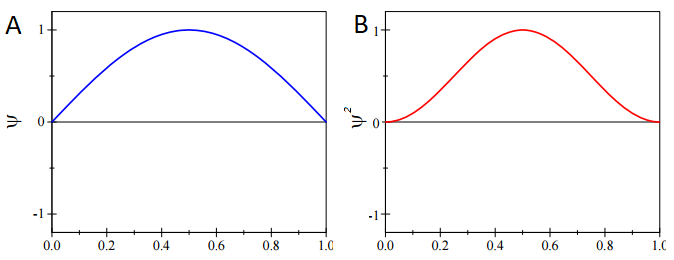
We can calculate the most probable position of the particle from knowledge of probability distribution, \(ψ^* ψ\). For the ground-state particle in a box wavefunction with \(n=1\) (Figure \(\PageIndex{1a}\))

\[\psi_{n=1} = \sqrt{\dfrac{2}{L}} \sin \left(\dfrac{\pi x}{L} \right) \label{PIB}\]

This state has the following probability distribution (Figure \(\PageIndex{1b}\)):

\[\psi^*_{n=1} \psi_{n=1} = \dfrac{2}{L} \sin^2 \left(\dfrac{\pi x}{L} \right)\]

Figure \(\PageIndex{1}\): (left) The ground-state (n=1) wavefunction for a particle in a box. (right) The ground-state (n=1) probability for a particle in a box.

The expectation value for position with the \(\hat{x} = x\) operation for any wavefunction (Equation \(\ref{expect}\)) is

\[ \langle x \rangle = \int _{-\infty}^{+\infty} \psi^* x \psi \, dx \]

which for the ground-state wavefunction (Equation \(\ref{PIB}\)) shown in Figure \(\PageIndex{1}\) is

\[ \begin{align} \langle x \rangle &= \int _{-\infty}^{+\infty} \sqrt{\dfrac{2}{L}} \sin \left(\dfrac{\pi x}{L} \right) x \sqrt{\dfrac{2}{L}} \sin \left(\dfrac{\pi x}{L} \right) \, dx \\[4pt] &= \dfrac{2}{L} \int _{-\infty}^{+\infty} x \sin^2 \left(\dfrac{\pi x}{L} \right) \label{GSExpect} \end{align}\]

Solution by Inspection

Without even having to evaluate Equation \(\ref{GSExpect}\), we can get the expectation value from simply inspecting \( \psi^*_{n=1} \psi_{n=1}\) in (Figure \(\PageIndex{1; right}\)). This is a symmetric distribution around the center of the box (\(L/2\)) so it is just as likely to be found in the left half than the right half) and more specifcally at any point away from the mean, i.e.

\[\psi^*_{n=1} \psi_{n=1} (L/2 + \Delta x) = \psi^*_{n=1} \psi_{n=1} (L/2 - \Delta x) \nonumber\]

Therefor, the particle is most likely to be found at the center of the box. So

\[ \langle x \rangle = \dfrac{L}{2} \nonumber \]

Exercise \(\PageIndex{4}\)

Use the general form of the particle-in-a-box wavefunction for any \(n\) to find the mathematical expression for the position expectation value \(\left \langle x \right \rangle\) for a box of length L. How does \(\left \langle x \right \rangle\) depend on \(n\)?

Average Momentum of a Particle in a Box

What is the average momentum of a particle in the box? We start with Equation \(\ref{expect}\) and use the momentum operator

\[\hat{p}_{x}=-i\hbar\dfrac{\partial}{\partial x}\label{3.2.3a}\]

We note that the particle-in-a-box wavefunctions are not eigenfunctions of the momentum operator (Exercise \(\PageIndex{4}\)). However, this does not mean that Equation \(\ref{expect}\) is inapplicable as Example \(\PageIndex{2}\) demonstrates.

Example \(\PageIndex{3}\): The Average Momentum of a Particle in a Box is Zero

Even though the wavefunctions are not momentum eigenfunctions, we can calculate the expectation value for the momentum. Show that the expectation or average value for the momentum of an electron in the box is zero in every state (i.e., arbitrary values of \(n\)).

Strategy

First write the expectation value integral (Equation \(\ref{expect}\)) with the momentum operator. Then insert the expression for the wavefunction and evaluate the integral as shown here.

Answer

\[\begin{align*} \left \langle p \right \rangle &= \int \limits ^L_0 \psi ^*_n (x) \left ( -i\hbar \dfrac {d}{dx} \right ) \psi _n (x) dx \\[4pt] &= \int \limits ^L_0 \left (\dfrac {2}{L} \right )^{1/2} \sin \left(\dfrac {n \pi x}{L}\right) \left ( -i\hbar \dfrac {d}{dx} \right ) \left (\dfrac {2}{L} \right )^{1/2} \sin \left(\dfrac {n \pi x }{L} \right) dx \\[4pt] &= -i \hbar \left (\dfrac {2}{L} \right ) \int \limits ^L_0 \sin \left(\dfrac {n \pi x}{L}\right) \left ( \dfrac {d}{dx} \right ) \sin \left(\dfrac {n \pi x}{L}\right) dx \\[4pt] &= -i \hbar \left (\dfrac {2}{L} \right ) \left ( \dfrac {n \pi}{L} \right ) \int \limits ^L_0 \sin \left(\dfrac {n \pi x}{L} \right) \cos \left(\dfrac {n \pi x}{L}\right) dx \\[4pt] &= 0 \end{align*} \]

Note that this makes sense since the particles spends an equal amount of time traveling in the \(+x\) and \(–x\) direction.

Interpretation

It may seem that this means the particle in a box does not have any momentum, which is incorrect because we know the energy is never zero. In fact, the energy that we obtained for the particle-in-a-box is entirely kinetic energy because we set the potential energy at 0. Since the kinetic energy is the momentum squared divided by twice the mass, it is easy to understand how the average momentum can be zero and the kinetic energy finite

Exercise \(\PageIndex{5}\)

Show that the particle-in-a-box wavefunctions are not eigenfunctions of the momentum operator (Equation \(\ref{3.2.3a}\)).

Answer

The easiest way to address this question is asking if the PIB wavefunction also satisfies the eigenvalue equation using the momentum operation instead of the Hamiltonian operator (3rd postulate of QM). That is

\[\hat{p}_x \psi(n) = p \psi(n) \nonumber\]

with

\[\psi_{n}=\sqrt{2 / L} \sin \left(\dfrac{n \pi x}{L}\right) \nonumber\]

and

\[\hat{p}=- i\hbar \dfrac{\partial}{\partial x } \nonumber\]

and \(p\) is a real scalar (since it is a measurable).

\[ \begin{align*} \hat{p}_x \psi_{n} &= - i\hbar \dfrac{\partial}{\partial x} \left[\sqrt{\dfrac{2}{L}} \sin \left(\dfrac{n \pi x}{L}\right)\right] \\[4pt] &= -i \hbar \sqrt{ \dfrac{2}{L}} \cos \left(\dfrac{n \pi x}{L}\right) \left(\dfrac{n \pi}{L}\right) \\[4pt] &\neq p \psi_{n} \end{align*}\]

Hence, the PIB wavefunctions are NOT eigenfunctions of the momentum operator.

It must be equally likely for the particle-in-a-box to have a momentum \(-p\) as \(+p\). The average of \(+p\) and \(–p\) is zero, yet \(p^2\) and the average of \(p^2\) are not zero. The information that the particle is equally likely to have a momentum of \(+p\) or \(–p\) is contained in the wavefunction. In fact, the sine function is a representation of the two momentum eigenfunctions \(e^{+ikx}\) and \(e^{-ikx}\) (Figure \(\PageIndex{2}\)).

Exercise \(\PageIndex{6}\)

Write the particle-in-a-box wavefunction as a normalized linear combination of the momentum eigenfunctions \(e^{ikx}\) and \(e^{-ikx}\) by using Euler’s formula. Show that the momentum eigenvalues for these two functions are \(p = +ħk\) and \(-ħk\).

The interpretation of the results of Exercise \(\PageIndex{6}\) is physically interesting. The exponential wavefunctions in the linear combination for the sine function represent the two opposite directions in which the electron can move. One exponential term represents movement to the left and the other term represents movement to the right (Figure \(\PageIndex{2}\)).

Figure \(\PageIndex{2}\): Two waves traveling in opposite directions across the same medium combine linearly. In this animation, both waves have the same wavelength and the sum of amplitudes results in a standing wave. (Public Domain; LucasVB).

The electrons are moving, they have kinetic energy and momentum, yet the average momentum is zero.

Did we just Violate the Uncertainty Principle?

Does the fact that the average momentum of an electron is zero and the average position is \(L/2\) violate the Heisenberg Uncertainty Principle? No, because the Heisenberg Uncertainty Principle pertains to the uncertainty in the momentum and in the position, not to the average values. Quantitative values for these uncertainties can be obtained to compare with the limit set by the Heisenberg Uncertainty Principle for the product of the uncertainties in the momentum and position. However, to do this we need a quantitative definition of uncertainty, which is discussed in the following Section.

Orthogonality

In vector calculus, orthogonality is the relation of two lines at right angles to one another (i.e., perpendicularity), but is generalized into \(n\) dimensions via zero amplitude "dot products" or "inner products." Hence, orthogonality is thought of as describing non-overlapping, uncorrelated, or independent objects of some kind. The concept of oethogonality extends to functions (wavefunctions or otherwise) too. Two functions \(\psi_A\) and \(\psi_B\) are said to be orthogonal if

\[ \int \limits _{all space} \psi _A^* \psi _B d\tau = 0 \label{3.7.3}\]

In general, eigenfunctions of a quantum mechanical operator with different eigenvalues are orthogonal. Are the eigenfunctions of the particle-in-a-box Hamiltonian orthogonal?

Exercise \(\PageIndex{7}\)

Evaluate the integral \(\int \psi ^*_1 \psi _3 dx\) for all possible pairs of particle-in-a-box eigenfunctions from \(n=1\) to \(n=3\) (use symmetry arguments whenever possible) and explain what the results say about orthogonality of the functions.

Contributors

• David M. Hanson, Erica Harvey, Robert Sweeney, Theresa Julia Zielinski ("Quantum States of Atoms and Molecules")