2.5: The Total Probability Sum at Constant N, V, and T

In a collection of distinguishable independent molecules at constant \(N\), \(V\), and \(T\), the probability that a randomly selected molecule has energy \({\epsilon }_i\) is \(P_i\); we have \(1=P_1+P_2+\dots +P_i+\dots\). At any instant, every molecule in the \(N\)-molecule system has a specific energy, and the state of the system is described by a population set, \(\{N_1,\ N_2,\dots ,N_i,\dots .\}\), wherein \(N_i\) can have any value in the range \(0\le N_i\le N\), subject to the condition that

\[N=\sum^{\infty }_{i=1}{N_i} \nonumber \]

The probabilities that we assume for this system of molecules have the properties we assume in Chapter 19 where we find the total probability sum by raising the sum of the energy-level probabilities to the \(N^{th}\) power.

\[1={\left(P_1+P_2+\dots +P_i+\dots \right)}^N=\sum_{\{N_i\}}{\frac{N!}{N_1!N_2!\dots N_i!\dots }}P^{N_1}_1P^{N_2}_2\dots P^{N_i}_i\dots \nonumber \]

The total-probability sum is over all possible population sets, \(\{N_1,\ N_2,\dots ,N_i,\dots .\}\), which we abbreviate to \(\{N_i\}\), in indicating the range of the summation. Each term in this sum represents the probability of the corresponding population set \(\{N_1,\ N_2,\dots ,N_i,\dots .\}\),. At any given instant, one of the possible population sets describes the way that the molecules of the physical system are apportioned among the energy levels. The corresponding term in the total probability sum represents the probability of this apportionment. It is not necessary that all of the energy levels be occupied. We can have \(N_k=0\), in which case \(P^{N_k}_k=P^0_k=1\) and \(N_k!=1\). Energy levels that are not occupied have no effect on the probability of a population set. The unique population set

\[\{N^{\textrm{⦁}}_1,\ N^{\textrm{⦁}}_2,\dots ,N^{\textrm{⦁}}_i,\dots .\} \nonumber \]

that we conjecture to characterize the equilibrium state is represented by one of the terms in this total probability sum. We want to focus on the relationship between a term in the total probability sum and the corresponding state of the physical system.

Each term in the total probability sum includes a probability factor, \(P^{N_1}_1P^{N_2}_2\dots P^{N_i}_i\dots\) This factor is the probability that \(N_i\) molecules occupy each of the energy levels \({\epsilon }_i\). This term is not affected by our assumption that the molecules are distinguishable. The probability factor is multiplied by the polynomial coefficient

\[\frac{N!}{N_1!N_2!\dots N_i!\dots } \nonumber \]

This factor is the number of combinations of distinguishable molecules that arise from the population set \(\{N_1,\ N_2,\dots ,N_i,\dots \}\). It is the number of ways that the \(N\) distinguishable molecules can be assigned to the available energy levels so that \(N_1\) of them are in energy level, \({\epsilon }_1\), etc.

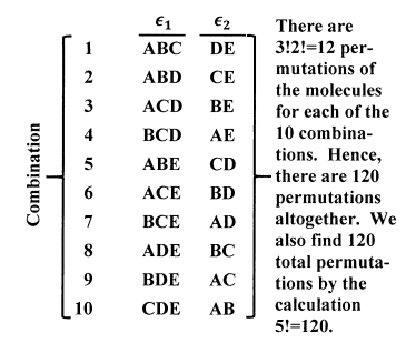
The combinations for the population set {3,2} are shown in Figure 2.

Figure 2. Combinations for the population set {3,2}.

The expression for the number of combinations takes the form it does only because the molecules can be distinguished from one another. To emphasize this point, let us find the number of combinations using the method we develop in Chapter 19. Briefly recapitulated, the argument is this:

1. We can permute the \(N\) molecules in \(N!\) ways. If we were to distinguish (as different combinations) any two permutations of all of the molecules, this would also be the number of combinations.
2. In fact, however, we do not distinguish between different permutations of those molecules that are assigned to the same energy level. If the \(N_1\) molecules assigned to the first energy level are \(B\), \(C\), \(Q\),…, \(X\), we do not distinguish the permutation \(BCQ\dots X\) from the permutation \(CBQ\dots X\) or from any other permutation of these \(N_1\) molecules. Then the complete set of \(N!\) permutations contains a subset of \(N_1!\) permutations, all of which are equivalent because they have the same molecules in the first energy level. So the total number of permutations, \(N!\), over-counts the number of combinations by a factor of \(N_1!\) We can correct for this over-count by dividing by \(N_1!\) That is, after correcting for the over-counting for the \(N_1\) molecules in the first energy level, the number of combinations is \({N!}/{N_1!}\) (If all \(N\) of the molecules were in the first energy level, there would be only one combination. We would have \(N=N_1\), and the number of combinations calculated from this formula would be \({N!}/{N!}=1\), as required.)
3. The complete set of \(N!\) permutations also includes \(N_2!\) permutations of the \(N_2\) molecules in the second energy level. In finding the number of combinations, we want to include only one of these permutations, so correcting for the over-counting due to both the \(N_1\) molecules in the first energy level and the \(N_2\) molecules in the second energy level gives \[\frac{N!}{N_1!N_2!} \nonumber \]
4. Continuing this argument through all of the occupied energy levels, we see that the total number of combinations is

\[C\left(N_1,N_2,\dots ,N_i,\dots \right)=\frac{N!}{N_1!N_2!\dots N_i!\dots } \nonumber \]

Because there are infinitely many energy levels and probabilities, \(P_i\), there are infinitely many terms in the total-probability sum. Every energy available to the macroscopic system is represented by one or more terms in this total-probability sum. Since there is no restriction on the energy levels that can be occupied, there are an infinite number of such system energies. There is an enormously large number of terms each of which corresponds to an enormously large system energy. Nevertheless, the sum of all of these terms must be one. The \(P_i\) form a convergent series, and the total probability sum must sum to unity.

Just as the \(P_i\) series can converge only if the probabilities of high molecular energies become very small, so the total probability sum can converge only if the probabilities of high system energies become very small. If a population set has \(N_i\) molecules in the \(i^{th}\) energy level, the probability of that population set is proportional to \(P^{N_i}_i\). We see therefore, that the probability of a population set in which there are many molecules in high energy levels must be very small. Terms in the total probability sum that correspond to population sets with many molecules in high energy levels must be negligible. Equivalently, at a particular temperature, macroscopic states in which the system energy is anomalously great must be exceedingly improbable.

What terms in the total probability sum do we need to consider? Evidently from among the infinitely many terms that occur, we can select a finite subset whose sum is very nearly one. If there are many terms that are small and nearly equal to one another, the number of terms in this finite subset could be large. Nevertheless, we can see that terms in this subset must involve the largest possible \(P_i\) values raised to the smallest possible powers, \(N_i\), consistent with the requirement that the \(N_i\) sum to \(N\).

If an equilibrium macroscopic system could have only one population set, the probability of that population set would be unity. Could an equilibrium system be characterized by two or more population sets for appreciable fractions of an observation period? Would this require that the macroscopic system change its properties with time as it jumps from one population set to another? Evidently, it would not, since our observations of macroscopic systems show that the equilibrium properties are unique. A system that wanders between two (or more) macroscopically distinguishable states cannot be at equilibrium. We are forced to the conclusion that, if a macroscopic equilibrium system has multiple population sets with non-negligible probabilities, the macroscopic properties associated with each of these population sets must be indistinguishably similar. (The alternative is to abandon the theory, which is useful only if its microscopic description of a system makes useful predictions about the system’s macroscopic behavior.)

To be a bit more precise about this, we recognize that our theory also rests on another premise: Any intensive macroscopic property of many independent molecules depends on the energy levels available to an individual molecule and the fraction of the molecules that populate each energy level. The average energy is a prime example. For the population set \(\{N_1,\ N_2,\dots ,N_i,\dots .\}\), the average molecular energy is

\[\overline{\epsilon }=\sum^{\infty }_{i=1}{\left(\frac{N_i}{N}\right)}{\epsilon }_i \nonumber \]

We recognize that many population sets may contribute to the total probability sum at equilibrium. If we calculate essentially the same \(\overline{\epsilon }\) from each of these contributing population sets, then all of the contributing population sets correspond to indistinguishably different macroscopic energies. We see in the next section that the central limit theorem guarantees that this happens whenever \(N\) is as large as the number of molecules in a macroscopic system.