1.24: Plug flow reactors and comparison to continuously stirred tank reactors
- Page ID
- 46936

Consider the following first-order irreversible reaction taking place in an adiabatic CSTR:
\[\text{A} \overset{k}{\longrightarrow} \text{B} + \text{C} \label{25.1}\]
Pure \(\text{A}\) is fed into the CSTR at a volumetric flow rate of \(10 \: \text{m}^3/\text{s}\) and a temperature, \(T_0 = 350 \: \text{K}\). The volume of the reactor is \(100 \: \text{m}^3\). What is the steady-state conversion, \(X\), and temperature, \(T\)? Additional information: \(C_{p, \text{A}} = 3 \: \text{J/mol} \cdot \text{K}\), \(C_{p, \text{B}} = 2 \: \text{J/mol} \cdot \text{K}\), \(C_{p, \text{C}} = 2 \: \text{J/mol} \cdot \text{K}\). \(\Delta H_\text{rxn} \left( 350 \: \text{K} \right) = -1500 \: \text{J/mol}\), \(E_a = 40,000 \: \text{J/mol}\), \(k = 1 \times 10^{-3} \: \text{s}^{-1}\) at \(T = 350 \: \text{K}\).
Solution
The design equation for a first-order irreversible reaction is given by
\[X = \frac{k \tau}{1 + k \tau} \label{25.2}\]
where
\[k \left( T \right) = k \left( 350 \: \text{K} \right) e^{-E_a \left( \frac{1}{RT} - \frac{1}{350 \: \text{K}} \right)} \label{25.3}\]
Combining the above expressions yields
\[X = \frac{k \left( 350 \: \text{K} \right) e^{_-E_a \left( \frac{1}{RT} - \frac{1}{350 \: \text{K}} \right)}}{1 + k \left( 350 \: \text{K} \right) e^{-E_a \left( \frac{1}{RT} - \frac{1}{350 \: \text{K}} \right)}} \label{25.4}\]
The energy balance for the CSTR can be written as
\[0 = F_{\text{A} 0} C_{p, \text{A}} \left( T_0 - T \right) - \left[ \Delta H_\text{rxn} \left( 350 \: \text{K} \right) + \Delta C_p \left( T - 350 \: \text{K} \right) \right] F_{\text{A} 0} X \label{25.5}\]
where \(\Delta C_p = C_{p, \text{C}} + C_{p, \text{B}} - C_{p, \text{A}}\). Rearranging in terms of \(X\) yields
\[X = \frac{C_{p, \text{A}} \left( T_0 - T \right)}{\Delta H_\text{rxn} \left( 350 \: \text{K} \right) + \Delta C_p \left( T - 350 \: \text{K} \right)} \label{25.6}\]
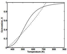
Equations \ref{25.4} and \ref{25.6} can be solved simultaneously for \(X\) and \(T\). Figure 25.1 displays plots of \(X\) versus \(T\) from Equation 25.4 (solid line) and Equation \ref{25.6} (dashed line). As can be seen from the figure, there are three combinations of \(X\) and \(T\) that will satisfy the two equations, indicating that there are multiple steady-states at which the reactor can operate.
Plug Flow Reactors (PFRs)
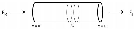
Another type of reactor used in industrial processes is the plug flow reactor (PFR). Like the CSTRs, a constant flow of reactants and products and exit the reactor. In PFRs, however, the reactor contents are not continuously stirred. Instead, chemical species are flowed along a tube as a plug, as shown in Figure 25.2. As the plug of fluid flows through the PFR, reactants are converted into products. In the diagram, \(F_{j 0} = F_j^\text{(in)}\), and \(F_j = F_j^\text{(out)}\).
PFRs are characterized by their length, \(L\), cross-sectional area, \(A\), and linear flow rate of fluids through the reactor, \(u\). For the purpose of our analysis, we will assume PFRs to be cylindrical, that there are no radial variations in the velocity, concentration, temperature or reaction rate along the reactor, and that there is no pressure drop or density variation along the reactor. Based on these assumptions, we can define the linear flow rate of fluid, \(u\), through the tube as
\[u = \frac{v}{A} \label{25.7}\]
where \(v\) is the volumetric flow rate and \(A\) is the cross-sectional area of the tube. The molar flow rate of species \(j\) along the reactor length can be defined in terms of \(u\) as
\[F_j \left( x, t \right) = v \left[ j \right] \left( x, t \right) = u A \left[ j \right] \left( x, t \right) \label{25.8}\]
where \(\left[ j \right]\) is a function of \(x\) and \(t\). Note that \(F_j \left( x, t \right)\) satisfies the boundary conditions:
\[\begin{align} F_j \left( 0, t \right) &= F_j^\text{(in)} \\ F_j \left( L, t \right) &= F_j^\text{(out)} \end{align} \label{25.9}\]
Mass balance for a PFR
As in the case of CSTRs, we can write a mass balance on species \(j\) in the PFR as
\[\left[ \text{accumulation of species} \: j \right] = \left[ \text{flow of species} \: j \: \text{in} \right] - \left[ \text{flow of species} \: j \: \text{out} \right] + \left[ \text{generation of species} \: j \right]\]
Because the concentration of species \(j\) varies along the length of the PFR, let us first consider a section of the PFR, \(\Delta x\). If \(\Delta x\) is sufficiently small, we can make the approximation that the reaction rate, \(r\), is constant within \(\Delta x\). We can the write the mass balance as
\[\frac{d N_j}{dt} = F_j \left( x, t \right) - F_j \left( x + \Delta x, t \right) + V \nu_j r_j \label{25.10}\]
where \(F_j \left( x, t \right)\) is the flow rate into the small volume, and \(F_j \left( x + \Delta x, t \right)\) is the flow rate out of the small volume. Since \(F_j \left( x, t \right) = u A \left[ j \right] \left( x, t \right)\) and \(F_j \left( x + \Delta x, t \right) = u A \left[ j \right] \left( x + \Delta x, t \right)\), we can write the mass balance condition as
\[\frac{d N_j}{dt} = V \frac{\partial \left[ j \right]}{\partial t} = A \Delta x \frac{\partial \left[ j \right]}{\partial t} = -A u \left( \left[ j \right] \left( x+ \Delta x, t \right) - \left[ j \right] \left( x, t \right) \right) + A \Delta x \nu_j r_j \label{25.11}\]
Now, we divide by \(A \Delta x\), which yields
\[\frac{\partial \left[ j \right]}{\partial t} = -u\left( \frac{\left[ j \right] \left( x + \Delta x, t \right) - \left[ j \right] \left( x, t \right)}{\Delta x} \right) + \nu_j r_j \label{25.12}\]
and if we take the limit \(\Delta x \rightarrow 0\), then the first term on the right becomes a spatial derivative, so that
\[\frac{\partial \left[ j \right]}{\partial t} + u \frac{\partial \left[ j \right]}{\partial x} = \nu_j r_j \label{25.13}\]
This constitutes a set of possibly coupled, nonlinear partial differential equations for all species in the reaction. The complexity of the equations is determined by the rate laws \(r_j\) for each species. If the rate laws are nonlinear, e.g., \(r_j = \pm k \left[ j \right]^{\nu_j}\) or involve multiple species, as occurs in complex reaction mechanisms, then the equations become rather complicated and need to be solved numerically.
However, let us suppose we can use a steady-state approximation so that \(\partial \left[ j \right]/\partial t = 0\). Then the equation becomes
\[\frac{d \left[ j \right]}{dx} = \frac{\nu_j}{u} r_j \label{25.14}\]
Examining Equation 25.14, we can see that the extent of conversion of reactants will depend on the length of the reactor, the linear flow rate, \(u\), and the reaction rate.
Fractional conversion in PFRs
For a first-order irreversible reaction in which \(\text{A} \rightarrow \text{B}\), the rate law is
\[r_\text{A} = -k \left[ \text{A} \right] \label{25.15}\]
and we can write Equation 25.14 as
\[\frac{d \left[ \text{A} \right]}{dx} = -\frac{1}{u} k \left[ \text{A} \right] \label{25.16}\]
Rearranging the above equation,
\[\int_{\left[ \text{A} \right]_0}^{\left[ \text{A} \right]} \frac{d \left[ \text{A} \right]}{\left[ \text{A} \right]} = -\frac{k}{u} \int_0^x dx' \label{25.17}\]
and integrating
\[\text{ln} \: \frac{\left[ \text{A} \right]_x}{\left[ \text{A} \right]_0} = -\frac{kx}{u} \label{25.18}\]
we can write the dependence of the concentration, \(\left[ \text{A} \right]\), along \(x\) as
\[\left[ \text{A} \right]_x = \left[ \text{A} \right]_0 e^{-\frac{kx}{u}} \label{25.19}\]
and the final concentration, \(\left[ \text{A} \right]_L\) as
\[\left[ \text{A} \right]_L = \left[ \text{A} \right]_0 e^{-\frac{kL}{u}} \label{25.20}\]
Recognizing that \(\frac{L}{u}\) is equal to the residence time, \(\tau\), for PFRs, we can also write the above equation as
\[\left[ \text{A} \right]_L = \left[ \text{A} \right]_0 e^{-k \tau} \label{25.21}\]
Plugging in
\[\left[ \text{A} \right]_L = \left[ \text{A} \right]_0 \left( 1 - X \right) \label{25.22}\]
we can also write the equation in terms of the fractional conversion
\[X = 1 - e^{-k \tau} \label{25.23}\]
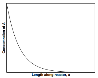
Figure 25.3 displays the concentration profile of species \(\text{A}\) along the length of the reactor. As can be seen from the figure, the concentration profile of species \(\text{A}\) in a PFR is identical to that in a batch reactor, with the exception that the \(x\)-axis is the length of the reactor instead of time. In fact, a PFR is a batch reactor in which we switch from a stationary coordinate system as a function of time to a moving coordinate system as function of distance, such that \(dt \rightarrow dx/u\). Thus,
\[\frac{d \left[ \text{A} \right]}{dt} \rightarrow u \frac{d \left[ \text{A} \right]}{dx} = -r \left( \left[ \text{A} \right] \right) \label{25.24}\]
Now consider a second-order reaction \(2 \: \text{A} \rightarrow \text{B}\). The rate law is
\[r_\text{A} = -k \left[ \text{A} \right]^2 \label{25.25}\]
Thus, the design equation gives the spatial profile of \(\text{A}\) as
\[\frac{d \left[ \text{A} \right]}{dx} = -\frac{2k}{u} \left[ \text{A} \right]^2 \label{25.26}\]
This can be solved in the same way that we solve the second-order rate kinetics.
\[\begin{align} \frac{d \left[ \text{A} \right]}{\left[ \text{A} \right]^2} &= -\frac{2k}{u} dx \\ -\frac{1}{\left[ \text{A} \right]} &= -\frac{2kx}{u} - C \\ \frac{1}{\left[ \text{A} \right]} &= \frac{2kx}{u} + C \\ \left[ \text{A} \right] \left( x \right) &= \frac{1}{\frac{2kx}{u} + C} \\ \left[ \text{A} \right] \left( 0 \right) &= \left[ \text{A} \right]_0 = \frac{1}{C} \\ C &= \frac{1}{\left[ \text{A} \right]_0} \\ \left[ \text{A} \right] \left( x \right) &= \frac{\left[ \text{A} \right]_0}{1 + \frac{2kx}{u} \left[ \text{A} \right]_0} \end{align} \label{25.27}\]
Thus, at the exit stream
\[\left[ \text{A} \right] \left( L \right) = \frac{\left[ \text{A} \right]_0}{1 + \frac{2kL}{u} \left[ \text{A} \right]_0} = \left[ \text{A} \right]_0 \left( 1 - X \right) \label{25.28}\]
This gives the conversion fraction as
\[X = \frac{2k \tau \left[ \text{A} \right]_0}{1 + 2k \tau \left[ \text{A} \right]_0} \label{25.29}\]
where \(\tau = L/u\) is the residence time.
Comparison of CSTRs and PFRs
For a first-order irreversible reaction, recall that the residence time, \(\tau\), for a CSTR is
\[\tau_\text{CSTR} = \frac{V_\text{CSTR}}{v} = \frac{\left[ \text{A} \right]_0 - \left[ \text{A} \right]}{k \left[ \text{A} \right]} \label{25.30}\]
while for a PFR, we can rearrange Equation 25.21 in terms of \(\tau\):
\[\tau_\text{PFR} = \frac{L_\text{PFR}}{u} = \frac{V_\text{PFR}}{v} = \frac{1}{k} \: \text{ln} \: \frac{\left[ \text{A} \right]_0}{\left[ \text{A} \right]} \label{25.31}\]
For equal volumetric flowrates into and out of the reactors, the ratio of the residence times of CSTRs and PFRs is equal to the ratio of the volumes of the reactors
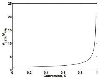
\[\frac{\tau_\text{CSTR}}{\tau_\text{PFR}} = \frac{V_\text{CSTR}}{V_\text{PFR}} = \frac{\left[ \text{A} \right]_0 - \left[ \text{A} \right]}{\left[ \text{A} \right] \: \text{ln} \left( \frac{\left[ \text{A} \right]_0}{\left[ \text{A} \right]} \right)} = \frac{X}{\left( 1 - X \right) \: \text{ln} \left( \frac{1}{1 - X} \right)} \label{25.32}\]
Figure 25.4 displays the plot of \(V_\text{CSTR}/V_\text{PFR}\) as a function of the fractional conversion, \(X\). As can be seen from the figure, the ratio is always positive, indicating that to achieve the same fractional conversion, the volume of a CSTR must be larger than the volume of a PFR. At high fractional conversion values, the volume required for a CSTR increases rapidly compared the the volume of a PFR. If reactor volume is the only criterion for deciding the type of reactor to use, clearly PFRs are the optimal choice. However, when one considers material costs and ease of operation, CSTRs may still be preferred for some applications.
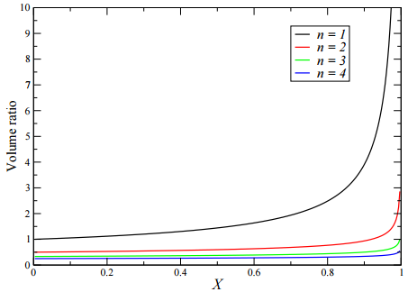
Despite Figure 25.4, there are other solutions to this problem. Consider a comparison of a PFR to \(n\) CSTRs in series. Recall that the conversion factor as a function of \(n\) for CSTRs in series is
\[X \left( n \right) = \frac{\left( 1 + k \tau \right)^n - 1}{\left( 1 + k \tau \right)^n} \label{25.33}\]
or
\[\begin{align} 1 &= \left( 1 + k \tau \right) \left( 1 - X \left( n \right) \right) \\ \left( 1 + k \tau \right) &= \left[ \frac{1}{1 - X \left( n \right)} \right]^{1/n} \\ k \tau &= \frac{1}{\left( 1 - X \left( n \right) \right)^{1/n}} - 1 \\ \tau &= \frac{1}{k} \left[ \frac{1 - \left( 1 - X \right)^{1/n}}{\left( 1 - X \right)^{1/n}} \right] \end{align} \label{25.34}\]
This gives
\[\frac{\tau_\text{CSTR, series}}{\tau_\text{PFR}} = \frac{V_\text{CSTR, series}}{V_\text{PFR}} = \frac{1 - \left( 1 - X \right)^{1/n}}{\left( 1 - X \right)^{1/n} \: \text{ln} \left( 1/ \left( 1 - X \right) \right)} \label{25.35}\]
If we now plot this ratio for different values of \(n\), we obtain the figure below: