1.10: Physical significance of free energy, Euler's theorem, Maxwell relations

Physical and Chemical Relevance of Free Energy

In this section, we will consider some examples showing the significance of free energies.

Drug binding

In pharmaceutical chemistry, free energies play a critical role in quantifying the strength of binding between an enzyme and an inhibitor such as a small-molecule inhibitor. An example of this is the use of the HIV-1 protease as a target for anti-AIDS therapies. The HIV-1 protease is a critical enzyme for the replication cycle of the AIDS virus, and numerous small-molecule inhibitors exist for arresting its catalytic function. An example is shown in the figure below: In designing such inhibitors, the binding process, itself, illustrated in the cartoon below is critical. This process

Figure 11.1: Illustration of a small molecule inhibitor complexed with the HIV-1 protease.

Figure 11.2: Cartoon illustrating the drug-enzyme binding process.

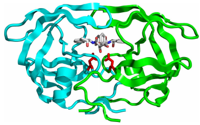
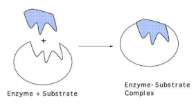
is an equilibrium between enzyme \(E\), inhibitor \(I\), and the bound complex \(EI\):

\[EI \leftrightharpoons E + I \label{11.1}\]

The equilibrium constant for this process

\[K = \frac{[E][I]}{[EI]} \equiv K_i \label{11.2}\]

is known as the inhibition constant. The smaller the value of \(K_i\), the greater the concentration of bound complexes, hence, the greater the strength of the binding. Optimal inhibitors of an enzyme have nanomolar or smaller \(K_i\) values. In general, the equilibrium constant for a process is determined by the change in the Gibbs free energy of the process. Hence, \(K_i\) is determined by the binding free energy process

\[\Delta G_\text{bind} = \Delta G(EI) - \Delta G(E) - \Delta G(I) \label{11.3}\]

so that

\[K_i = e^{\beta \Delta G_\text{bind}} \label{11.4}\]

Solvation free energies

As the previous example showed, the binding free energy quantifies the strength of the interaction between a drug and a target enzyme. While this is a critical component of the drug design process, another process of key importance is solubility. Most medications are formulated as tablets or gel capsules, both of which contain small crystalline particles. These crystalline particles must be water soluble in order for them to be bioavailable. The solvation process for a substance \(A\) is captured in the reaction

\[A(g) \leftrightharpoons A(aq) \label{11.5}\]

and illustrated humorously below: The equilibrium constant for this process \(K_\text{solv}\) is also determined by the solvation

Figure 11.3: Illustration of the solvation process.

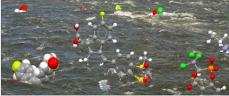
Gibbs free energy \(\Delta G_\text{solv}\):

\[K_\text{solv} = e^{-\beta \Delta G_\text{solv}} \label{11.6}\]

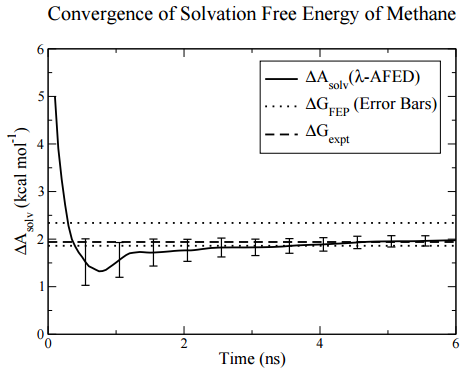
As an example of calculation of \(\Delta G_\text{solv}\) and \(\Delta A_\text{solv}\), the plot below shows a computer simulation of the solvation of methane in water, in which solvated configurations are sampling via molecular dynamics (numerical solution of Newton’s equations of motion), and an algorithm designed to speed the convergence with simulation time of the free energy is employed. The convergence of \(\Delta A_\text{solv}\) is compared to experiment and known theoretical values of \(\Delta G_\text{solv}\). In this case, it can be seen that \(\Delta G_\text{solv}\) and \(\Delta A_\text{solv}\) are nearly identical.

Configurational Free Energies

Free energies can be used to characterize the conformational preferences and the conformational equilibria of complex molecules. Such free energies can be useful, for example, in understanding the process of protein or polypeptide folding. An example of the folding of an alanine decamer into an alpha-helix is shown below. The folding process can be characterized in terms of a particular mechanical coordinate in the system known as a reaction coordinate, and the free energy along such a coordinate can be mapped out in order to obtain free energy differences between

Figure 11.4: Convergence of a calculation of \(\Delta A_\text{solv}\) for methane in water and comparison to the experimental value.

Figure 11.5: Folding pathway of an alanine decamer.

Figure 11.6: Typical folding free energy curve.

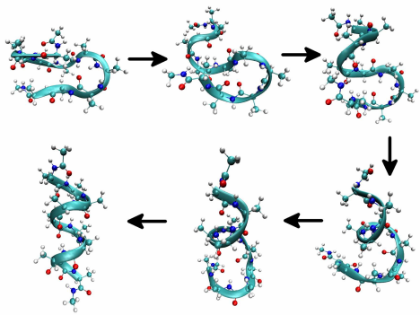
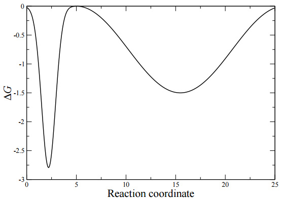
unfolded, partially folded, and fully folded conformations. For folding, a useful coordinate is the root-mean square deviation (RMSD) from the fully folded state of the alpha carbons along the peptide backbone. A typical free energy map of this type appears as in the figure below. The free energy curve shows a narrow and deep minimum at small values of the reaction coordinate, here the RMSD from the folded conformation. This deep minimum is associated with the folded state. The wide basin at large values of the RMSD corresponds to metastable intermediates, which are misfolded states and \(\beta\)-hairpin type conformations.

Free Energies of Crystalline Polymorphs

Polymorphism refers to the ability of certain small organic molecules to form numerous distinct crystal structures. This is a critical problem in the pharmaceutical industry, where most medications are administered in crystalline form. Hence, if a particular compound is able to convert from a metastable, soluble crystal to a highly stable, insoluble form, while the medication sits on the shelf, is a serious problem that can lead to expensive recalls. A priori prediction of crystalline polymorphs of small molecules is, therefore, a problem of critical importance. Computational prediction of polymorphs can play an important role in this endeavor, and the development of such techniques is an outstanding grand challenge problem. A successful prediction of polymorphs should also include a thermodynamic ranking of these structures, and such a ranking should be based on the relative free energy of the polymorphs. An example of the polymorphs of benzene at \(100\) K and \(2\) GPa pressure is shown in the figure below along with the unit cells of each crystal structure. The figure shows free energies (green curve), simple lattice energies at \(0\) K (red curve), and

Figure 11.7: Relative free energies of the polymorphs of solid benzene.

the relative populations of different polymorphs (blue bars). The figure suggests that the Benzene III polymorph is thermodynamically the most stable structure under the conditions reported above.

Euler's Theorem

Recall the definition of the Helmholtz free energy is \(A = E - TS\), hence, a change in \(A\) at constant temperature is

\[\Delta A = \Delta E - T \Delta S \label{11.7}\]

Since \(T \Delta S = \Delta Q_\text{rev}\), we obtain

\[\Delta A = \Delta E - \Delta Q_\text{rev} \label{11.8}\]

which means that

\[\Delta A = \Delta W_\text{rev} \label{11.9}\]

Hence, the change in the Helmholtz free energy in an isothermal process is equal to the reversible work performed on the system in the process.

There is another way to obtain this relation that involves a very general property of many thermodynamic functions. This property is a consequence of a theorem known as Euler’s Theorem. Euler’s theorem is a general statement about a certain class of functions known as homogeneous functions of degree \(n\). Consider a function \(f(x_1, \ldots, x_N)\) of \(N\) variables that satisfies

\[f(\lambda x_1, \ldots, \lambda x_k, x_{k+1}, \ldots, x_N) = \lambda^n f(x_1, \ldots, x_k, x_{k+1}, \ldots, x_N) \label{11.10}\]

for an arbitrary parameter, \(\lambda\). We call such a function a homogeneous function of degree \(n\) in the variables \(x_1, \ldots, x_k\). The function \(f(x) = x^2\), for example, is a homogeneous function of degree \(2\). The function \(f(x, y, z) = xy^2 + z^3\) is a homogeneous function of degree \(3\) in all three variables \(x\), \(y\), and \(z\). The function \(f(x, y, z) = x^2 (y^2 + z)\) is a homogeneous function of degree \(2\) in \(x\) but not in \(y\) and \(z\). The function \(f(x, y) = e^{xy} - xy\) is not a homogeneous function in either \(x\) or \(y\).

Euler’s theorem states the following: Let \(f(x_1, \ldots, x_N)\) be a homogeneous function of degree \(n\) in \(x_1, x_k\). Then,

\[nf(x_1, \ldots, x_N) = \sum_{i=1}^k x_i \frac{\partial f}{\partial x_i} \label{11.11}\]

The proof of Euler’s theorem is straightforward. Beginning with Equation 11.10, we differentiate both sides with respect to \(\lambda\) to yield:

\[\begin{align} \frac{d}{d \lambda} f(\lambda x_1, \ldots, \lambda x_k, x_{k+1}, \ldots, x_N) &= \frac{d}{d \lambda} \lambda^n f(x_1, \ldots, x_k, x_{k+1}, \ldots, x_N) \\ \sum_{i=1}^k x_i \frac{\partial f}{\partial (\lambda x_i)} &= n \lambda^{n-1} f(x_1, \ldots, x_k, x_{k+1}, \ldots, x_N) \end{align} \label{11.12}\]

Since \(\lambda\) is arbitrary, we may freely choose \(\lambda = 1\), which yields

\[\sum_{i=1}^k x_i \frac{\partial f}{\partial x_i} = nf(x_1, \ldots, x_k, x_{k+1}, \ldots, x_N) \label{11.13}\]

and proves the theorem.

What does Euler’s theorem have to do with thermodynamics? Consider, for example, the Helmholtz free energy \(A (N, V, T)\), which depends on two extensive variables, \(N\) and \(V\). Since \(A\) is, itself, extensive, \(A \sim N\), and since \(V \sim N\), \(A\) must be a homogeneous function of degree \(1\) in \(N\) and \(V\), i.e. \(A(\lambda N, \lambda V, T) = \lambda A(N, V, T)\). Applying Euler’s theorem, it follows that

\[A(N, V, T) = V \frac{\partial A}{\partial V} + N \frac{\partial A}{\partial N} \label{11.14}\]

From the thermodynamic relations of the canonical ensemble for pressure and chemical potential, we have \(P = -(\partial A/ \partial V)\) and \(\mu = (\partial A/ \partial N)\). Thus,

\[A = -PV + \mu N \label{11.15}\]

We can verify this result by recalling that

\[A(N, V, T) = E - TS \label{11.16}\]

From the first law of thermodynamics,

\[E - TS = -PV + \mu N \label{11.17}\]

so that

\[A(N, V, T) = -PV + \mu N \label{11.18}\]

which agrees with Euler’s theorem. Now, a small change in \(A\) under reversible conditions gives

\[dA = -P(V) \: dV + \mu (N) \: dN \label{11.19}\]

which is a general expression for the reversible work done on a system when both volume and number of particles (or moles) changes. In fact, any extensive thermodynamic quantity must be a homogeneous function of degree \(1\) in its extensive arguments.

Thus, the Gibbs free energy \(G(N, P, T)\) is a homogeneous function of degree \(1\) in \(N\). Hence, we can write

\[G = N \frac{\partial G}{\partial N} = \mu N \label{11.20}\]

Thus, \(dG = \mu (N) \: dN\), and the quantity \(dG + P \: dV = G + P_\text{ext} \: dV\) is the reversible work performed on a system under isobaric conditions.

Maxwell Relations

Free energies provide a route to relating changes in thermodynamic derivatives, i.e., changes in certain thermodynamic quantities under different conditions. These useful relations are not always obvious but can be easily derived starting from either a Helmholtz or Gibbs free energy. Unlike the relations of the previous section, the relations we will consider next emerge from second derivatives of the free energy functions and are referred to as Maxwell relations after the 19th Century Scottish physicist James Clerk Maxwell, who also developed the classical theory of electromagnetic fields (in the form of the celebrated Maxwell equations). We will see that the first derivative relations of the previous section, however, provide the starting point.

Consider the Helmholtz free energy \(A = E - TS\). In a process that changes temperature and energy (and, therefore, the entropy as well), the free energy change is

\[dA = dE - S \: dT - T \: dS \label{11.21}\]

From the first law, \(dE = -P \: dV + T \: dS\), hence

\[dA = -P \: dV + T \: dS - S \: dT - T \: dS = -P \: dV - S \: dT \label{11.22}\]

However, by the chain rule, if \(N\) remains fixed

\[dA = \left( \frac{\partial A}{\partial V} \right)_T dV + \left( \frac{\partial A}{\partial T} \right)_V dT \label{11.23}\]

Equating these two relations, we find

\[P = -\left( \frac{\partial A}{\partial V} \right)_T, \: \: \: \: \: \: \: S = -\left( \frac{\partial A}{\partial T} \right)_V \label{11.24}\]

It is trivially obvious that

\[\frac{\partial^2 A}{\partial V \partial T} = \frac{\partial^2 A}{\partial T \partial V} \label{11.25}\]

However, the above relation tells us that

\[\left(\frac{\partial P}{\partial T} \right)_V = \left( \frac{\partial S}{\partial V} \right)_T \label{11.26}\]

which is an example of a Maxwell relation. It tells us how to compute the change in entropy with respect to volume from a knowledge of the equation of state. If we integrate both sides, the entropy change when the volume changes from \(V_1\) to \(V_2\) is

\[\Delta S = \int_{V_1}^{V_2} \left( \frac{\partial P}{\partial T} \right)_V dV \label{11.27}\]

Thus, for an ideal gas, \(P = nRT/V\), \(\partial P/ \partial T = nR/V\), hence,

\[\Delta S = nR \int_{V_1}^{V_2} \frac{dV}{V} = nR \: \text{ln} \: \left( \frac{V_2}{V_1} \right) \label{11.28}\]

If \(N\) is allowed to change as well, then the Equations 11.22 and 11.23 must be modified to read

\[\begin{align} dA &= - P \: dV + \mu \: dN - S \: dT \\ dA &= \left( \frac{\partial A}{\partial N} \right)_{V, T} dN \left( \frac{\partial A}{\partial V} \right)_{N, T} dV + \left( \frac{\partial A}{\partial T} \right)_{N, V} dT \end{align} \label{11.29}\]

so that

\[\mu = \left( \frac{\partial A}{\partial N} \right)_{V, T} \label{11.30}\]

Think about the additional Maxwell relations that can be derived from this relation for the chemical potential.

If we start with the Gibbs free energy instead, and consider the second derivative of \(G\) with respect to \(N\) and \(P\) under isothermal conditions, we obtain another useful Maxwell relation

\[\begin{align} \frac{\partial ^ G}{\partial N \partial P} &= \frac{\partial^2 G}{\partial P \partial N} \\ \frac{\partial \mu}{\partial P} &= \frac{\partial \langle V \rangle}{\partial N} \end{align} \label{11.31}\]

which tells us that the change in chemical pressure with respect to pressure is equal to the change in the average volume with respect to the number of particles or the number of moles.