1.5: The van der Waals equation of state and radial distribution functions
- Page ID
- 44108

The Van der Waals Equation of State
In the last lecture, we saw that for the pair potential
\[u(r) = \begin{cases} \infty & r \leq \sigma \\ -\dfrac{C_6}{r^6} & r > \sigma \end{cases} \label{\(\PageIndex{1}\)}\]
we could write the second virial coefficient as
\[B_2(T) = \dfrac{2}{3} \pi N_0 \sigma^3 \left[ 1 - \dfrac{C_6}{3 k_B T \sigma^6} \right] \label{\(\PageIndex{2}\)}\]
Let us introduce to simplifying variables
\[\begin{align} b &= \dfrac{2}{3} \pi N_0 \sigma^3 \\ a &= \dfrac{2 \pi N_0^2 C_6}{9 \sigma^3} \end{align} \label{\(\PageIndex{3}\)}\]
in terms of which
\[B_2(T) = b - \dfrac{a}{RT} \label{\(\PageIndex{4}\)}\]
With these definitions, the virial equation of state becomes
\[\begin{align} P &= \dfrac{nRT}{V} + \dfrac{n^2}{V^2} RT \left( b - \dfrac{a}{RT} \right) \\ &= \dfrac{nRT}{V} \left(1 + \dfrac{nb}{V} \right) - \dfrac{an^2}{V^2} \end{align} \label{\(\PageIndex{5}\)}\]
If we assume \(nb/V\) is small, then we can also write
\[1 + \dfrac{nb}{V} \approx \dfrac{1}{1 - \dfrac{nb}{V}} \label{\(\PageIndex{6}\)}\]
so that
\[P = \dfrac{nRT}{V - nb} - \dfrac{an^2}{V^2} \label{\(\PageIndex{7}\)}\]
which is known as the van der Waals equation of state.

The first term in this equation is easy to motivate. In fact, it looks very much like the equation of state for an ideal gas having volume \(V - nb\) rather than \(V\). This part of the van der Waals equation is due entirely to the hard-wall potential \(u_o(r)\). Essentially, this potential energy term describes a system of “billiard balls” of diameter \(\sigma\). The figure below shows two of these billiard ball type particles at the point of contact (also called the distance of closest approach). At this point, they undergo a collision and separate, so that cannot be closer than the distance shown in the figure. At this point, the distance between their centers is also \(\sigma\), as the figure indicates. Because of this distance of closest approach, the total volume available to the particles is not \(V\) but some volume less than \(V\). This reduction in volume can be calculated as follows: Figure \(\PageIndex{1}\) shows a shaded sphere that just contains the pair of billiard ball particles. The volume of this sphere is the volume excluded from any two particles. The radius of the sphere is \(\sigma\) as the figure shows. Hence, the excluded volume for the two particles is \(4 \pi \sigma^3/3\), which is the volume of the shaded sphere. From this, we see that the excluded volume for any one particle is just half of this or \(2 \pi \sigma^3/3\). The excluded volume for a mole of such particles is just \(2 \pi \sigma^3 N_0/3\), which is the parameter \(b\):
\[b = \dfrac{2}{3} \pi \sigma^3 N_0 \label{\(\PageIndex{8}\)}\]
Given \(n\) moles of gas, the total excluded volume is then \(nb\), so that the total available volume is simply \(V - nb\).
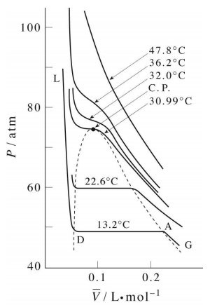
Isotherms of the van der Waals equation are shown in the figure below (left panel). In the figure the volume axis is the molar volume denoted \(\bar{V} = V/n\). At sufficiently high temperature, the isotherms approach those of an ideal gas. However, we also see something strange in some of the isotherms. Specifically, we see a region in which \(P\) and \(V\) increase together, and we know that this cannot actually happen in a real gas. It should be clear that many approximations and assumptions go into the derivation of the van der Waals equation so that some of the important physics is missing from the model. Hence, we should not be surprised if the van der Waals equation has some unphysical behavior buried in it.
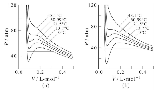
In fact, we know that at sufficiently low temperatures, any real gas, when compressed, must undergo a transition from gas to liquid. The signature of such a transition is a discontinuous change in the volume, signifying the condensation of the gas into a liquid that occupies a significantly lower volume. Unfortunately, the van der Waals equation does not correctly predict this behavior, and hence, it must be added in ad hoc. This is done by drawing a horizontal line through the isotherm (Figure \(\PageIndex{2}\)) and in the figure below. The vertical position of the line is
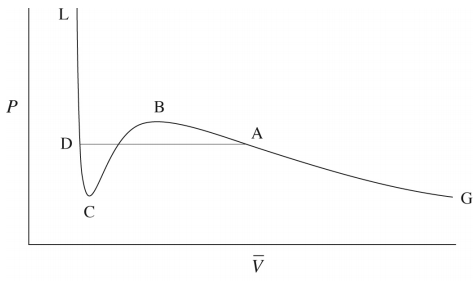
chosen so that the area above the line (between the line and the isotherm) and below the line (again between the line and the isotherm) is exactly the same. In this way, we entirely remove the artifact of the unphysical increase of \(P\) with \(V\) when we compute the compressional work on the gas from \(\int P(V) \: dV\), to be discussed in our section on thermodynamics. This horizontal line is called the tie line.
As it happens, there is exactly one isotherm along which the van der Waals equation correctly predicts the gas-to-liquid phase transition. Along this isotherm, the volume discontinuity captured by the tie line is shrunken down to a single point (so that there is no possibility of an increase of \(P\) with \(V\)!). This isotherm, in fact, corresponds to the highest possible temperature at which such a transition can occur. As we approach this isotherm from higher temperatures, this isotherm is a kind of dividing line between the system’s remaining a gas at all value of \(P\) and \(V\) and the system’s actually undergoing a gas-to-liquid transition. Hence, this isotherm is called the critical isotherm (Figure \(\PageIndex{4}\)): The temperature of this isotherm is called the critical temperature, denoted \(T_c\). The point at which the curve flattens out, signifying the phase transition, is called the critical point. If we draw a curve through the isotherms joining all points of these isotherms at which the tie lines begin, continue the curve up to the critical isotherm, and down the other side where the tie lines end, this curve reaches a maximum at the critical point. This is illustrated below:
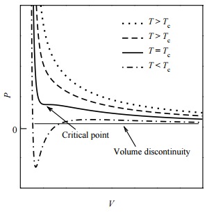
The shape of the critical isotherm at the critical point allows us to determine the exact temperature, pressure, and volume at which the phase transition from gas to liquid will occur. At this point, the isotherm is both horizontal and flat. This means that both the first and second derivatives of \(P\) with respect to \(V\) must vanish:
\[\dfrac{\partial P}{\partial V} = 0, \: \: \: \dfrac{\partial^2 P}{\partial V^2} = 0 \label{\(\PageIndex{9}\)}\]
Substituting the van der Waals equation into these two conditions, we find the following:
\[\begin{align} -\dfrac{nRT}{\left( V - nb \right)^2} + \dfrac{2 an^2}{V^3} &= 0 \\ \dfrac{2nRT}{\left( V - nb \right)^3} - \dfrac{6an^2}{V^4} &= 0 \end{align} \label{\(\PageIndex{1}\)0}\]
Hence, we have two equations in two unknowns \(V\) and \(T\) for the critical temperature and critical volume. Once these are determined, the van der Waals equation, itself, allows us to determine the critical pressure.
To solve the equations, first divide one by the other. This gives us a simple condition for the volume:
\[\begin{align} \dfrac{V - nb}{2} &= \dfrac{V}{3} \\ 3V - 3nb &= 2V \\ V &= 3nb \equiv V_c \end{align} \label{\(\PageIndex{1}\)1}\]
This is the critical volume. Now use either of the two conditions to obtain the critical temperature \(T_c\). If we use the first one, we find
\[\begin{align} \dfrac{nRT_c}{\left( V_c - nb \right)^2} &= \dfrac{2an^2}{V_c^3} \\ \dfrac{nRT_c}{\left( 3nb - nb \right)^2} &= \dfrac{2an^2}{\left( 3nb \right)^3} \\ \dfrac{nRT_c}{4n^2b^2} &= \dfrac{2an^2}{27n^3b^3} \\ RT_c &= \dfrac{8a}{27b} \end{align} \label{\(\PageIndex{1}\)2}\]
Finally, plugging the critical temperature and volume into the van der Waals equation, we obtain the critical pressure
as
\[\begin{align} P &= \dfrac{nRT_c}{V_c - nb} - \dfrac{an^2}{V_c^2} \\ &= \dfrac{8an/27b}{3nb - nb} - \dfrac{an^2}{\left( 3nb \right)^2} \\ &= \dfrac{a}{27b^2} \end{align} \label{\(\PageIndex{1}\)3}\]
Structure of Liquids
Characterizing the structure and thermodynamics of liquids is obviously more challenging than it is for gases because the types of approximations that work for gases do not for liquids, and we need to take into account the full set of interactions in constructing the partition function. Although there are analytical theories that have been developed for liquids (such as integral-equation theory, one of the developers of which is our Jerome Percus at the Courant Institute), these theories have largely been supplanted by computer simulations, which yield more accurate results and can be applied to liquids of essentially any complexity.
In terms of statistical mechanics, one of the most important quantities used to characterize the nature of the liquid 6 state is the co-called radial distribution function or pair correlation function. It is denoted \(g(r)\) and is defined to be
\[g(r) = \dfrac{\left( N - 1 \right)}{4 \pi \rho r^2} \dfrac{1}{Z} \int_{| \textbf{r}_1 - \textbf{r}_2 | = r} dx_{\textbf{r}} \: e^{-\beta U \left( \textbf{r}_1, \ldots, \textbf{r}_N \right)} \label{\(\PageIndex{1}\)4}\]
where
\[Z = \int dx_{\textbf{r}} \: e^{-\beta U \left( \textbf{r}_1, \ldots, \textbf{r}_N \right)} \label{\(\PageIndex{1}\)5}\]
is the configurational partition function. Physically, the quantity \(r^2 g(r) \: dr\) gives us the fraction of particles or the probability that a particle is in a spherical shell of thickness \(dr\) at a distance \(r\) from another particle. Because of attractive forces between particles in liquids, each particle in a liquid tends to be surrounded by a “shell” of other particles at some average distance. This shell is called a solvation shell or coordination shell or, when the liquid is water, a hydration shell. Particles in this solvation shell also have their own solvation shells, and these have solvation shells, and so forth. Thus, a liquid can actually exhibit a surprising amount of structure, and the function \(g(r)\) captures that structure very clearly. Moreover, \(g(r)\) is a function that can be measured experimentally using the techniques of neutron or X-ray scattering in a setup that is somewhat analogous to Bragg scattering from crystals. Recall that Bragg scattering is used to measure the distance between crystalline planes in a solid. In a liquid, the particles are in constant motion, so there are no well-defined distances, however, certain average distance values are favored over others, and these scattering experiments capture these average distances just as Bragg scattering experiments capture more fixed distances in solids.
Figure \(\PageIndex{6}\) shows the radial distribution functions for liquid argon at several different temperatures. Not only can we see
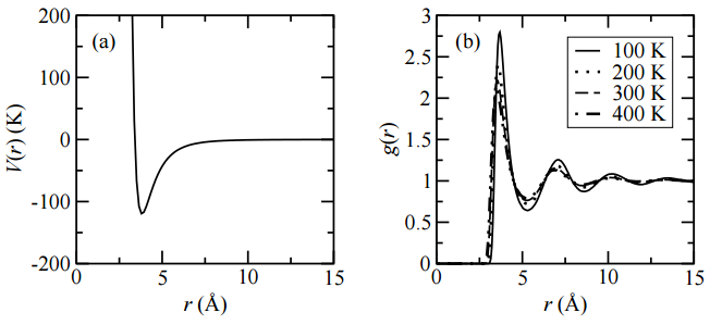
the existence of several solvation shells, we can read off the plot the distances at which these solvation shells peak around a central atom in the liquid. From the plot, we clearly see that \(g(r)\) is a function of temperature and depends sensitively on it. In particular, as temperature increases, structure tends to decrease.
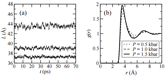
In the same way, Figure \(\PageIndex{7}\) shows that the radial distribution function also depends on pressure. We see the same liquid argon system subject to several pressures. Even though the volume fluctuations (see panel on the left) tend to be small, pressure changes somewhat the degree of structuring in the liquid. In particular, as we compress the liquid, it tends to become more structured, as we might expect. At higher pressures, particles are less likely to escape from solvation shells and tend to fluctuate less within these solvation shells.
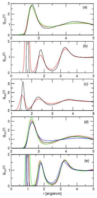
Finally, we show the three radial distribution functions of water, including computer simulation results and the experimental results from neutron scattering and X-ray scattering. In the case of the computer simulations, the
calculations are performed using a technique known as ab initio or first-principles molecular dynamics. In this approach, the forces and potential energies for each nuclear configuration are generated by direct solution of the Schrödinger equation (based on the approximation of density functional theory). This allows to generate these functions with absolutely no experimental input parameters – they really do come from first principles.