
1.13: The Clapeyron equation, Gibbs phase rule, and Classical Nucleation Theory
- Page ID
- 45509

The Clapeyron Equation
The Clapeyron attempts to answer the question of what the shape of a two-phase coexistence line is. In the \(P-T\) plane, we see the a function \(P(T)\), which gives us the dependence of \(P\) on \(T\) along a coexistence curve.
Consider two phases, denoted \(\alpha\) and \(\beta\), in equilibrium with each other. These could be solid and liquid, liquid and gas, solid and gas, two solid phases, et. Let \(\mu_\alpha (P, T)\) and \(\mu_\beta (P, T)\) be the chemical potentials of the two phases. We have just seen that
\[\mu_\alpha (P, T) = \mu_\beta (P, T) \label{14.1}\]
Next, suppose that the pressure and temperature are changed by \(dP\) and \(dT\). The changes in the chemical potentials of each phase are
\[ d \mu_{\alpha} (P, T) = d \mu_{\beta} (P, T) \label{14.2a}\]
\[\left( \dfrac{\partial \mu_{\alpha}}{\partial P} \right)_T dP + \left( \dfrac{\partial \mu_{\alpha}}{\partial T} \right)_P dT = \left( \dfrac{\partial \mu_{\beta}}{\partial P} \right)_T dP + \left( \dfrac{\partial \mu_{\beta}}{\partial T} \right)_P dT \label{14.2b}\]
However, since \(G(n, P, T) = n \mu (P, T)\), the molar free energy \(\bar{G} (P, T)\), which is \(G(n, P, T)/n\), is also just equal to the chemical potential
\[\bar{G} (P, T) = \dfrac{G(n, P, T)}{n} = \mu (P, T) \label{14.3}\]
Moreover, the derivatives of \(\bar{G}\) are
\[\left( \dfrac{\partial \bar{G}}{\partial P} \right)_T = \bar{V}, \: \: \: \: \: \: \: \left( \dfrac{\partial \bar{G}}{\partial T} \right)_P = -\bar{S} \label{14.4}\]
Applying these results to the chemical potential condition in Equation \(\ref{14.2b}\), we obtain
\[\begin{align} \left( \dfrac{\partial \bar{G}_\alpha}{\partial P} \right)_T dP + \left( \dfrac{\partial \bar{G}_\alpha}{\partial T} \right)_P dT &= \left( \dfrac{\partial \bar{G}_\beta}{\partial P} \right)_T dP + \left( \dfrac{\partial \bar{G}_\beta}{\partial T} \right)_P dT \
\[5pt] \bar{V}_\alpha dP - \bar{S}_\alpha dT &= \bar{V}_\beta dP - \bar{S}_\beta dT \end{align} \label{14.5}\]
Dividing through by \(dT\), we obtain
\[\begin{align} \bar{V}_\alpha \dfrac{\partial P}{\partial T} - \bar{S}_\alpha &= \bar{V}_\beta \dfrac{\partial P}{\partial T} - \bar{S}_\beta \
\[5pt] (\bar{V}_\alpha - \bar{V}_\beta) \dfrac{\partial P}{\partial T} &= \bar{S}_\alpha - \bar{S}_\beta \
\[5pt] \dfrac{dP}{dT} &= \dfrac{\bar{S}_\alpha - \bar{S}_\beta}{\bar{V}_\alpha - \bar{V}_\beta} \end{align} \label{14.6}\]
The importance of the quantity \(dP/dT\) is that is represents the slope of the coexistence curve on the phase diagram between the two phases. Now, in equilibrium \(dG = 0\), and since \(G = H - TS\), it follows that \(dH = T \: dS\) at fixed \(T\). In the narrow temperature range in which the two phases are in equilibrium, we can assume that \(H\) is independent of \(T\), hence, we can write \(S = H/T\). Consequently, we can write the molar entropy difference as
\[\bar{S}_\alpha - \bar{S}_\beta = \dfrac{\bar{H}_\alpha - \bar{H}_\beta}{T} \label{14.7}\]
and the pressure derivative \(dP/dT\) becomes
\[\dfrac{dP}{dT} = \dfrac{\bar{H}_\alpha - \bar{H}_\beta}{T (\bar{V}_\alpha - \bar{V}_\beta)} = \dfrac{\Delta_{\alpha \beta} \bar{H}}{T \Delta_{\alpha \beta} \bar{V}} \label{14.8}\]
a result known as the Clapeyron equation, which tells us that the slope of the coexistence curve is related to the ratio of the molar enthalpy between the phases to the change in the molar volume between the phases. If the phase equilibrium is between the solid and liquid phases, then \(\Delta_{\alpha \beta} \bar{H}\) and \(\Delta_{\alpha \beta} \bar{V}\) are \(\Delta \bar{H}_\text{fus}\) and \(\Delta \bar{V}_\text{fus}\), respectively. If the phase equilibrium is between the liquid and gas phases, then \(\Delta_{\alpha \beta} \bar{H}\) and \(\Delta_{\alpha \beta} \bar{V}\) are \(\Delta \bar{H}_\text{vap}\) and \(\Delta \bar{V}_\text{vap}\), respectively.
For the liquid-gas equilibrium, some interesting approximations can be made in the use of the Clapeyron equation. For this equilibrium, Equation \(\ref{14.8}\) becomes
\[\dfrac{dP}{dT} = \dfrac{\Delta \bar{H}_\text{vap}}{T (\bar{V}_g - \bar{V}_l)} \label{14.9}\]
In this case, \(\bar{V}_g \gg \bar{V}_l\), and we can approximate Equation \(\ref{14.9}\) as
\[\dfrac{dP}{dT} \approx \dfrac{\Delta \bar{H}_\text{vap}}{T \bar{V}_g} \label{14.10}\]
Suppose that we can treat the vapor phase as an ideal gas. Certainly, this is not a good approximation so close to the vaporization point, but it leads to an example we can integrate. Since \(PV_g = nRT\), \(P \bar{V}_g = RT\), Equation \(\ref{14.10}\) becomes
\[\begin{align} \dfrac{dP}{dT} &= \dfrac{\Delta \bar{H}_\text{vap} P}{RT^2} \
\[5pt] \dfrac{1}{P} \dfrac{dP}{dT} &= \dfrac{\Delta \bar{H}_\text{vap}}{RT^2} \
\[5pt] \dfrac{d \: \text{ln} \: P}{dT} &= \dfrac{\Delta \bar{H}_\text{vap}}{RT^2} \end{align} \label{14.11}\]
which is called the Clausius-Clapeyron equation. We now integrate both sides, which yields
\[\text{ln} \: P = -\dfrac{\Delta \bar{H}_\text{vap}}{RT} + C\]
where \(C\) is a constant of integration. Exponentiating both sides, we find
\[P(T) = C' e^{-\Delta \bar{H}_\text{vap}/RT}\]
which actually has the wrong curvature for large \(T\), but since the liquid-vapor coexistence line terminates in a critical point, as long as \(T\) is not too large, the approximation leading to the above expression is not that bad.
If we, instead, integrate both sides, the left from \(P_1\) to \(P_2\), and the right from \(T_1\) to \(T_2\), we find
\[\begin{align} \int_{P_1}^{P_2} d \: \text{ln} \: P &= \int_{T_1}^{T_2} \dfrac{\Delta \bar{H}_\text{vap}}{RT^2} dT \
\[5pt] \text{ln} \: \left( \dfrac{P_2}{P_1} \right) &= -\dfrac{\Delta \bar{H}_\text{vap}}{R} \left( \dfrac{1}{T_2} - \dfrac{1}{T_1} \right) \
\[5pt] &= \dfrac{\Delta \bar{H}_\text{vap}}{R} \left( \dfrac{T_1 - T_1}{T_1 T_2} \right) \end{align} \label{14.12}\]
assuming that \(\Delta \bar{H}_\text{vap}\) is independent of \(T\). Here \(P_1\) is the pressure of the liquid phase, and \(P_2\) is the pressure of the vapor phase. Suppose we know \(P_2\) at a temperature \(T_2\), and we want to know \(P_3\) at another temperature \(T_3\). The above result can be written as
\[\text{ln} \: \left( \dfrac{P_3}{P_1} \right) = -\dfrac{\Delta \bar{H}_\text{vap}}{R} \left( \dfrac{1}{T_3} - \dfrac{1}{T_1} \right) \label{14.13}\]
Subtracting the two results, we obtain
\[\text{ln} \: \left( \dfrac{P_2}{P_3} \right) = -\dfrac{\Delta \bar{H}_\text{vap}}{R} \left( \dfrac{1}{T_2} - \dfrac{1}{T_3} \right) \label{14.14}\]
so that we can determine the vapor pressure at any temperature if it is known as one temperature.
In order to illustrate the use of this result, consider the following example:
At \(1 \: \text{bar}\), the boiling point of water is \(373 \: \text{K}\). At what pressure does water boil at \(473 \: \text{K}\)? Take the heat of vaporization of water to be \(40.65 \: \text{kJ/mol}\).
Solution
Let \(P_1 = 1 \: \text{bar}\) and \(T_1 = 373 \: \text{K}\). Take \(T_2 = 473 \: \text{K}\), and we need to calculate \(P_2\). Substituting in the numbers, we find
\[\begin{align} \text{ln} \: P_2(\text{bar}) &= -\dfrac{(40.65 \: \text{kJ/mol})(1000 \: \text{J/kJ})}{8.3145 \: \text{J/mol} \cdot \text{K}} \left( \dfrac{1}{473 \: \text{K}} - \dfrac{1}{373 \: \text{K}} \right) = 2.77 \
\[5pt] P_2(\text{bar}) &= (1 \: \text{bar}) \: e^{2.77} = 16 \: \text{bar} \end{align}\]
Gibbs Phase Rule
In any one-component system with three phases, there is only one point at which all three phases coexist in equilibrium. This is known as the triple point. Although the Gibbs free energy \(G\) is a function of \(n\), \(P\), and \(T\), \(G = G(n, P, T)\), if we allow ourselves to treat \(P\) and \(T\) as experimental control parameters, as is done when we construct a phase diagram, then \(n\) is determined by the equation of state. \(P\) and \(T\) are both intensive properties.
Now suppose we have a multicomponent system. When we have more than one component, we have additional intensive properties that could potentially be additional degrees of freedom that determine the dimensionality of the phase diagram. If the phase diagram has a dimensionality higher than that of a plane (two dimensions), then triple points could become lines, planes, curved surfaces, or hypersurfaces. Thus, it is important to have a way of determining how many actual experimental control variables we have in a multicomponent system. This number is determined by the number of thermodynamic conditions that exist among the intensive properties. We will now derive a relation that accounts for these conditions and yields the total number of degrees of freedom or experimental control parameters – this relation is known as the Gibbs phase rule.
Suppose a system has \(k\) components and can exist in \(p\) phases. An example would be a three-component system consisting of \(H_2O\), \(CH_3OH\), and \(CH_3CH_2OH\). The Gibbs free energy \(G\) is now a function of \(n_1, \ldots, n_k\), \(P\), and \(T\): \(G = G(n_1, \ldots, n_k, P, T)\). The total number of moles \(n\) is still determined by the equation of state if we allow \(P\) and \(T\) to be experimental control parameters. However, we now have a condition
\[n_1 + n_2 + \cdots + n_k = n \label{14.15}\]
We can now introduce additional intensive parameters by dividing both sides by \(n\), which yields
\[\dfrac{n_1}{n} + \dfrac{n_2}{n} + \cdots + \dfrac{n_k}{n} = 1 \label{14.16}\]
We defined
\[X^{(i)} = \dfrac{n_1}{n} \label{14.17}\]
called the mole fraction of component \(i\). Clearly, we must have
\[X^{(1)} + X^{(2)} + \cdots + X^{(k)} = 1\]
Moreover, \(X^{(i)}\) is an intensive property.
Suppose, for starters, that \(k = 1\), but we have \(p\) phases. If \(\alpha\) and \(\beta\) denote a pair of phases, then at a \(p\)-phase coexistence point, we have a set of conditions from the chemical potential equalization that take the form
\[\mu_\alpha (P, T) = \mu_\beta (P, T) \label{14.18}\]
For example, if we had three phases, solid, liquid, and gas, the conditions would be
\[\mu_\text{liq} (P, T) = \mu_\text{gas} (P, T), \: \: \: \: \: \: \: \mu_\text{liq} (P, T) = \mu_\text{solid} (P, T), \: \: \: \: \: \: \: \mu_\text{solid} (P, T) = \mu_\text{gas} (P, T) \label{14.19}\]
However, by the transitive property, the third condition follows from the first two, so it’s not an independent condition. In fact, we have only two independent conditions. In general, if we have \(p\) phases, we have \(p - 1\) such conditions.
Now if we have \(k\) components, then we have \(p - 1\) such conditions for each phase, giving a total of \(k(p - 1)\) total conditions from chemical potential equalization. The fact that the mole fractions in each phase must sum to \(1\) gives us additional condition. Let \(X_\alpha^{(i)}\) be the mole fraction of component \(i\) in phase \(\alpha\). For each phase, we have a condition
\[X_\alpha^{(1)} + X_\alpha^{(2)} + \cdots + X_\alpha^{(k)} = 1 \label{14.20}\]
This gives us \(p\) additional conditions. Hence, the total number of conditions we have is \(k(p - 1) + p\). Although the equation of state constitutes, in principle, another condition, we have already taken it into account by positing that the total number of moles \(n\) is determined if we know \(P\) and \(T\).
Now the total number of mole fractions is \(k\) for each phase for a total of \(kp\) mole fractions. In addition, if we add \(P\) and \(T\) as additional parameters, then the total number of intensive thermodynamic parameters we can tune is \(kp + 2\). If we subtract from this the number of conditions (also the number of constraints), we obtain the number of degrees of freedom \(d\) as
\[\begin{array}{rcl} d & = & kp + 2 - k(p - 1) - p \
\[5pt] & = & kp + 2 - kp + k - p \
\[5pt] & = & k - p + 2 \end{array}\]
The condition
\[d = k - p + 2 \label{14.21}\]
is known as the Gibbs phase rule.
As an example, suppose we have \(k = 3\) components and \(p = 3\) phases. Then the number of degrees of freedom is
\[d = 3 - 3 + 2 = 2\]
which we could take to be \(P\) and \(T\). However, we could also take these to be \(P\) and one of the mole fractions or \(T\) and one of the mole fractions.
As another example, consider water, which has three phases, ice, water, steam. Here, we have \(k = 1\) and \(p = 3\). Thus,
\[d = 1 - 3 + 2 = 0\]
which means that when all three phases are in coexistence, the number of degrees of freedom is \(0\). Hence, there can be only one point, i.e. one value of \(P\) and one value of \(T\), at which this coexistence occurs, which we call the triple point. However, this explains why the triple point is a point and not a structure of higher dimension.
Classical Nucleation Theory
Having looked at phase diagrams in some detail, we now turn our attention to the process by which phase transitions occur. In particular, we will consider a phenomenological theory known as classical nucleation theory. Let us consider it in the special case of the solid-liquid transition, i.e., the melting transition. In this case, if we are in the solid phase and far from the melting point, then we have the condition \(\mu_s < \mu_l\), which tells us that the solid phase is more stable (remember that chemical potentials are also molar free energies, and the solid phase should have a lower free energy far from the melting point).
As we approach the melting point, the liquid phase becomes the more stable of the two phases, and we have \(\mu_s > \mu_l\) or \(\mu_l - \mu_s < 0\). The solid phase now becomes a metastable phase. This means that, even though the liquid phase is the more stable of the two phases, there is a significant free energy barrier that must be crossed in order for the system to undergo a transition from solid to liquid. How do we characterize this barrier? In order to do this, we introduce a microscopic coordinate in the system that is capable of following the progress of the melting process. Such a coordinate is called a reaction coordinate. In general, a reaction coordinate is some function of the atomic positions that is capable of following a particular process, such as chemical reaction, a diffusion process, or a phase transition.
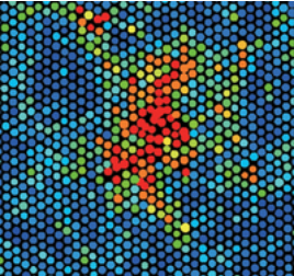
Classical nucleation theory (CNT) posits that as a solid is heated close to its melting point, a liquid nucleus can form in the solid, and as this nucleus grows, eventually, the system will melt completely, transforming from solid to liquid. If we assume that this nucleus is a sphere of radius \(r\), then \(r\) can be viewed as the reaction coordinate. As \(r\) increases, the size of the liquid nucleus increases, and ultimately, the system melts. This process is illustrated in Figure 14.1 below.
The free energy to form a nucleus of radius \(r\) will be a function of \(r\), which we denote as \(\Delta G(r)\). Such a coordinate-dependent free energy is called a free energy profile. The free energy needed to form such a nucleus has two contributions. First, work is needed to form the surface of the nucleus, which is an interface between the solid and the liquid. As these two things do not naturally fit together, it is not energetically favorable to form the surface of the nucleus. Let \(\gamma_s\) denote the surface tension of the nucleus, which has units of energy per unit area. The area of the nucleus is \(4 \pi r^2\), so this contribution to the free energy is \(4 \pi r^2 \gamma_s\). On the other hand, since \(\mu_l < \mu_s\), forming a liquid nucleus of volume \(4 \pi r^3/3\) is favorable. If \(\Delta \mu\) represents the chemical potential difference per unit volume, then given that \(\Delta \mu < 0\), this contribution to the free energy \((4 \pi r^3/3) \Delta \mu\) is negative. Hence, we have a balance between the volume and surface area terms, and the total free energy in the CNT is
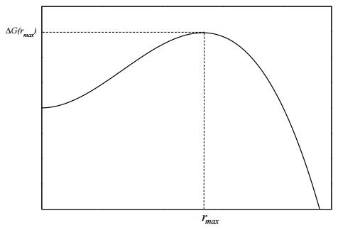
\[\Delta G(r) = \dfrac{4}{3} \pi r^3 \Delta \mu + 4 \pi r^2 \gamma_s \label{14.22}\]
If we plot this free energy as a function of \(r\), we obtain a curve of the form show in Figure 14.2. We see from the free energy profile that there is a significant barrier at a particular radius \(r_\text{max}\). The height of the barrier is \(\Delta G(r_\text{max})\). To find what this radius is, we need to maximize \(\Delta G\). We take the derivative of \(\Delta G(r)\) with respect to \(r\) and set it equal to \(0\)
\[\begin{align} \dfrac{d \Delta G}{dr} = 4 \pi r^2 \Delta \mu + 8 \pi r \gamma_s &= 0 \
\[5pt] r \Delta \mu + 2 \gamma_s &= 0 \
\[5pt] r &= - \dfrac{2 \gamma_s}{\Delta \mu} \equiv r_\text{max} \end{align} \label{14.23}\]
If we evaluate the free energy at this radius, we find the barrier height to be
\[\begin{align} \Delta G(r_\text{max}) &= \dfrac{4}{3} \pi \left( - \dfrac{2 \gamma_s}{\Delta \mu} \right)^3 + 4 \pi \left( -\dfrac{2 \gamma_s}{\Delta \mu} \right)^2 \gamma_s \
\[5pt] &= -\dfrac{4}{3} \pi \left( \dfrac{8 \gamma_s^3}{(\Delta \mu)^3} \right) \Delta \mu + 4 \pi \left( \dfrac{4 \gamma_s^2}{(\Delta \mu)^2} \right) \gamma_s \
\[5pt] &= \dfrac{16 \pi \gamma_s^3}{3 (\Delta \mu)^2} \end{align} \label{14.24}\]
For water, for example, the height of the barrier, computed from this formula, would be around \(100 k_B T\), which corresponds to a barrier of around \( 50 \: \text{kcal/mol}\). Thus, we see that, although the liquid phase is more stable, a very high energy barrier needs to be surmounted, which is a rare event.