4.4: Molecular Structure and Polarity

Learning Objectives

• Predict the structures of small molecules using valence shell electron pair repulsion (VSEPR) theory
• Explain the concepts of polar covalent bonds and molecular polarity
• Assess the polarity of a molecule based on its bonding and structure

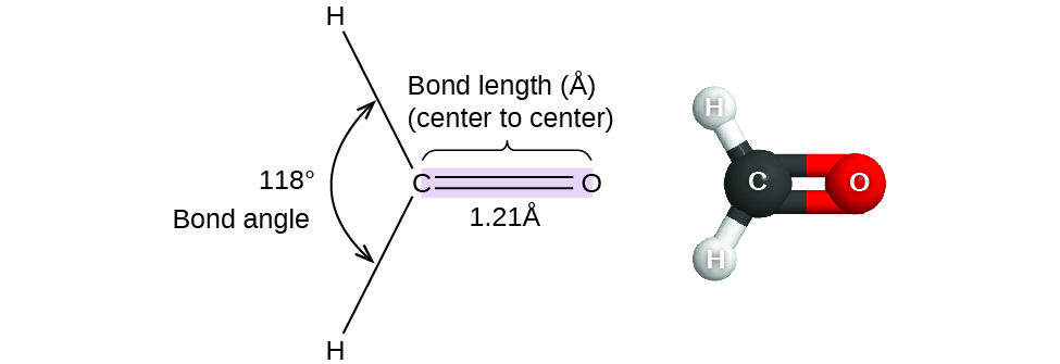
Thus far, we have used two-dimensional Lewis structures to represent molecules. However, molecular structure is actually three-dimensional, and it is important to be able to describe molecular bonds in terms of their distances, angles, and relative arrangements in space (Figure \(\PageIndex{1}\)). A bond angle is the angle between any two bonds that include a common atom, usually measured in degrees. A bond distance (or bond length) is the distance between the nuclei of two bonded atoms along the straight line joining the nuclei. Bond distances are measured in Ångstroms (1 Å = 10^–10 m) or picometers (1 pm = 10^–12 m, 100 pm = 1 Å).

Figure \(\PageIndex{1}\): Bond distances (lengths) and angles are shown for the formaldehyde molecule, H₂CO.

VSEPR Theory

Valence shell electron-pair repulsion theory (VSEPR theory) enables us to predict the molecular structure, including approximate bond angles around a central atom, of a molecule from an examination of the number of bonds and lone electron pairs in its Lewis structure. The VSEPR model assumes that electron pairs in the valence shell of a central atom will adopt an arrangement that minimizes repulsions between these electron pairs by maximizing the distance between them. The electrons in the valence shell of a central atom form either bonding pairs of electrons, located primarily between bonded atoms, or lone pairs. The electrostatic repulsion of these electrons is reduced when the various regions of high electron density assume positions as far from each other as possible.

VSEPR theory predicts the arrangement of electron pairs around each central atom and, usually, the correct arrangement of atoms in a molecule. We should understand, however, that the theory only considers electron-pair repulsions. Other interactions, such as nuclear-nuclear repulsions and nuclear-electron attractions, are also involved in the final arrangement that atoms adopt in a particular molecular structure.

As a simple example of VSEPR theory, let us predict the structure of a gaseous BeF₂ molecule. The Lewis structure of BeF₂ (Figure \(\PageIndex{2}\)) shows only two electron pairs around the central beryllium atom. With two bonds and no lone pairs of electrons on the central atom, the bonds are as far apart as possible, and the electrostatic repulsion between these regions of high electron density is reduced to a minimum when they are on opposite sides of the central atom. The bond angle is 180° (Figure \(\PageIndex{2}\)).

Figure \(\PageIndex{2}\): The BeF₂ molecule adopts a linear structure in which the two bonds are as far apart as possible, on opposite sides of the Be atom.

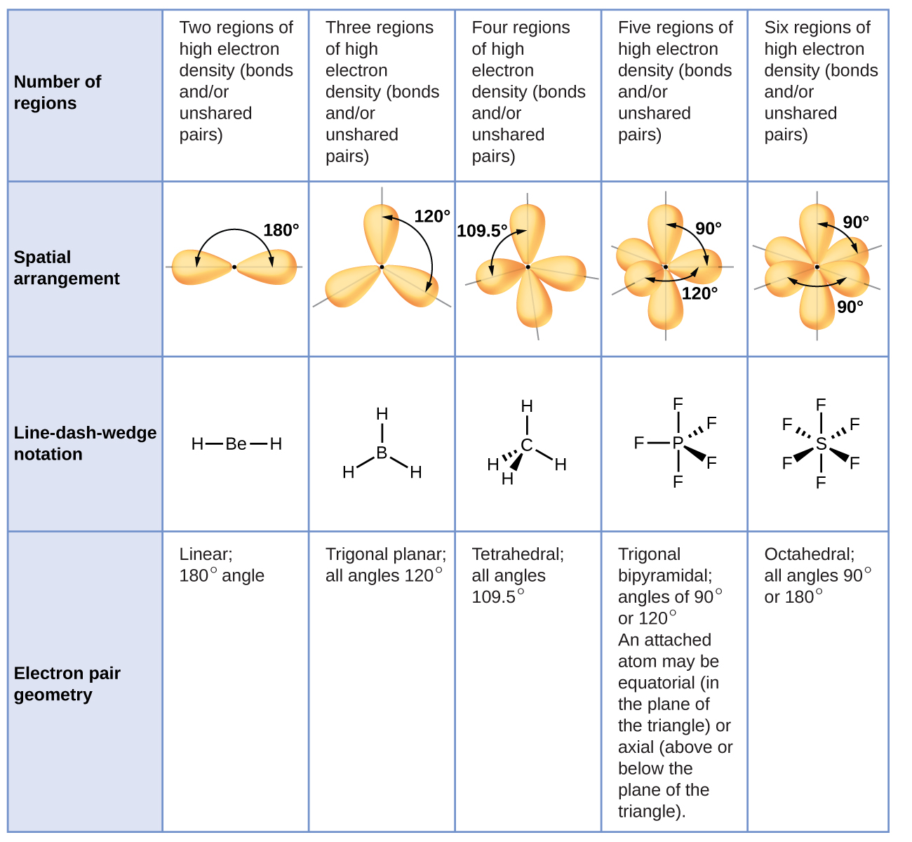
Figure \(\PageIndex{3}\) illustrates this and other electron-pair geometries that minimize the repulsions among regions of high electron density (bonds and/or lone pairs). Two regions of electron density around a central atom in a molecule form a linear geometry; three regions form a trigonal planar geometry; four regions form a tetrahedral geometry; five regions form a trigonal bipyramidal geometry; and six regions form an octahedral geometry.

Figure \(\PageIndex{3}\): The basic electron-pair geometries predicted by VSEPR theory maximize the space around any region of electron density (bonds or lone pairs).

Electron-pair Geometry versus Molecular Structure

It is important to note that electron-pair geometry around a central atom is not the same thing as its molecular structure. The electron-pair geometries shown in Figure \(\PageIndex{3}\) describe all regions where electrons are located, bonds as well as lone pairs. Molecular structure describes the location of the atoms, not the electrons.

We differentiate between these two situations by naming the geometry that includes all electron pairs the electron-pair geometry. The structure that includes only the placement of the atoms in the molecule is called the molecular structure. The electron-pair geometries will be the same as the molecular structures when there are no lone electron pairs around the central atom, but they will be different when there are lone pairs present on the central atom.

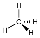
Figure \(\PageIndex{4}\): The molecular structure of the methane molecule, CH₄, is shown with a tetrahedral arrangement of the hydrogen atoms. VSEPR structures like this one are often drawn using the wedge and dash notation, in which solid lines represent bonds in the plane of the page, solid wedges represent bonds coming up out of the plane, and dashed lines represent bonds going down into the plane.

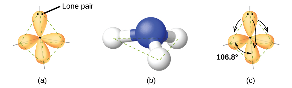
For example, the methane molecule, CH₄, which is the major component of natural gas, has four bonding pairs of electrons around the central carbon atom; the electron-pair geometry is tetrahedral, as is the molecular structure (Figure \(\PageIndex{4}\)). On the other hand, the ammonia molecule, NH₃, also has four electron pairs associated with the nitrogen atom, and thus has a tetrahedral electron-pair geometry. One of these regions, however, is a lone pair, which is not included in the molecular structure, and this lone pair influences the shape of the molecule (Figure \(\PageIndex{5}\)).

Figure \(\PageIndex{5}\): (a) The electron-pair geometry for the ammonia molecule is tetrahedral with one lone pair and three single bonds. (b) The trigonal pyramidal molecular structure is determined from the electron-pair geometry. (c) The actual bond angles deviate slightly from the idealized angles because the lone pair takes up a larger region of space than do the single bonds, causing the HNH angle to be slightly smaller than 109.5°.

Small distortions from the ideal angles in Figure \(\PageIndex{5}\) can result from differences in repulsion between various regions of electron density. VSEPR theory predicts these distortions by establishing an order of repulsions and an order of the amount of space occupied by different kinds of electron pairs. The order of electron-pair repulsions from greatest to least repulsion is:

lone pair-lone pair > lone pair-bonding pair > bonding pair-bonding pair

This order of repulsions determines the amount of space occupied by different regions of electrons. A lone pair of electrons occupies a larger region of space than the electrons in a triple bond; in turn, electrons in a triple bond occupy more space than those in a double bond, and so on. The order of sizes from largest to smallest is:

lone pair > triple bond > double bond > single bond

Consider formaldehyde, H₂CO, which is used as a preservative for biological and anatomical specimens. This molecule has regions of high electron density that consist of two single bonds and one double bond. The basic geometry is trigonal planar with 120° bond angles, but we see that the double bond causes slightly larger angles (121°), and the angle between the single bonds is slightly smaller (118°).

In the ammonia molecule, the three hydrogen atoms attached to the central nitrogen are not arranged in a flat, trigonal planar molecular structure, but rather in a three-dimensional trigonal pyramid (Figure \(\PageIndex{6}\)) with the nitrogen atom at the apex and the three hydrogen atoms forming the base. The ideal bond angles in a trigonal pyramid are based on the tetrahedral electron pair geometry. Notice that since we are only examining compounds that obey the octet rule, we'll only be using rows 2, 3, and 4 in this figure. The ideal molecular structures are predicted based on the electron-pair geometries for various combinations of lone pairs and bonding pairs.

Figure \(\PageIndex{6}\): The molecular structures are identical to the electron-pair geometries when there are no lone pairs present (first column). For a particular number of electron pairs (row), the molecular structures for one or more lone pairs are determined based on modifications of the corresponding electron-pair geometry.

According to VSEPR theory, the terminal atom locations (Xs in Figure \(\PageIndex{7}\)) are equivalent within the linear, trigonal planar, and tetrahedral electron-pair geometries (the first three rows of the table). It does not matter which X is replaced with a lone pair because the molecules can be rotated to convert positions.

Predicting Electron Pair Geometry and Molecular Structure

The following procedure uses VSEPR theory to determine the electron pair geometries and the molecular structures:

1. Write the Lewis structure of the molecule or polyatomic ion.
2. Count the number of regions of electron density (lone pairs and bonds) around the central atom. A single, double, or triple bond counts as one region of electron density.
3. Identify the electron-pair geometry based on the number of regions of electron density: linear, trigonal planar, tetrahedral, trigonal bipyramidal, or octahedral (Figure \(\PageIndex{7}\), first column).
4. Use the number of lone pairs to determine the molecular structure (Figure \(\PageIndex{7}\) ). If more than one arrangement of lone pairs and chemical bonds is possible, choose the one that will minimize repulsions, remembering that lone pairs occupy more space than multiple bonds, which occupy more space than single bonds. In trigonal bipyramidal arrangements, repulsion is minimized when every lone pair is in an equatorial position. In an octahedral arrangement with two lone pairs, repulsion is minimized when the lone pairs are on opposite sides of the central atom.

The following examples illustrate the use of VSEPR theory to predict the molecular structure of molecules or ions that have no lone pairs of electrons. In this case, the molecular structure is identical to the electron pair geometry.

Example \(\PageIndex{1}\): Predicting Electron-pair Geometry and Molecular Structure

Predict the electron-pair geometry and molecular structure for the following:

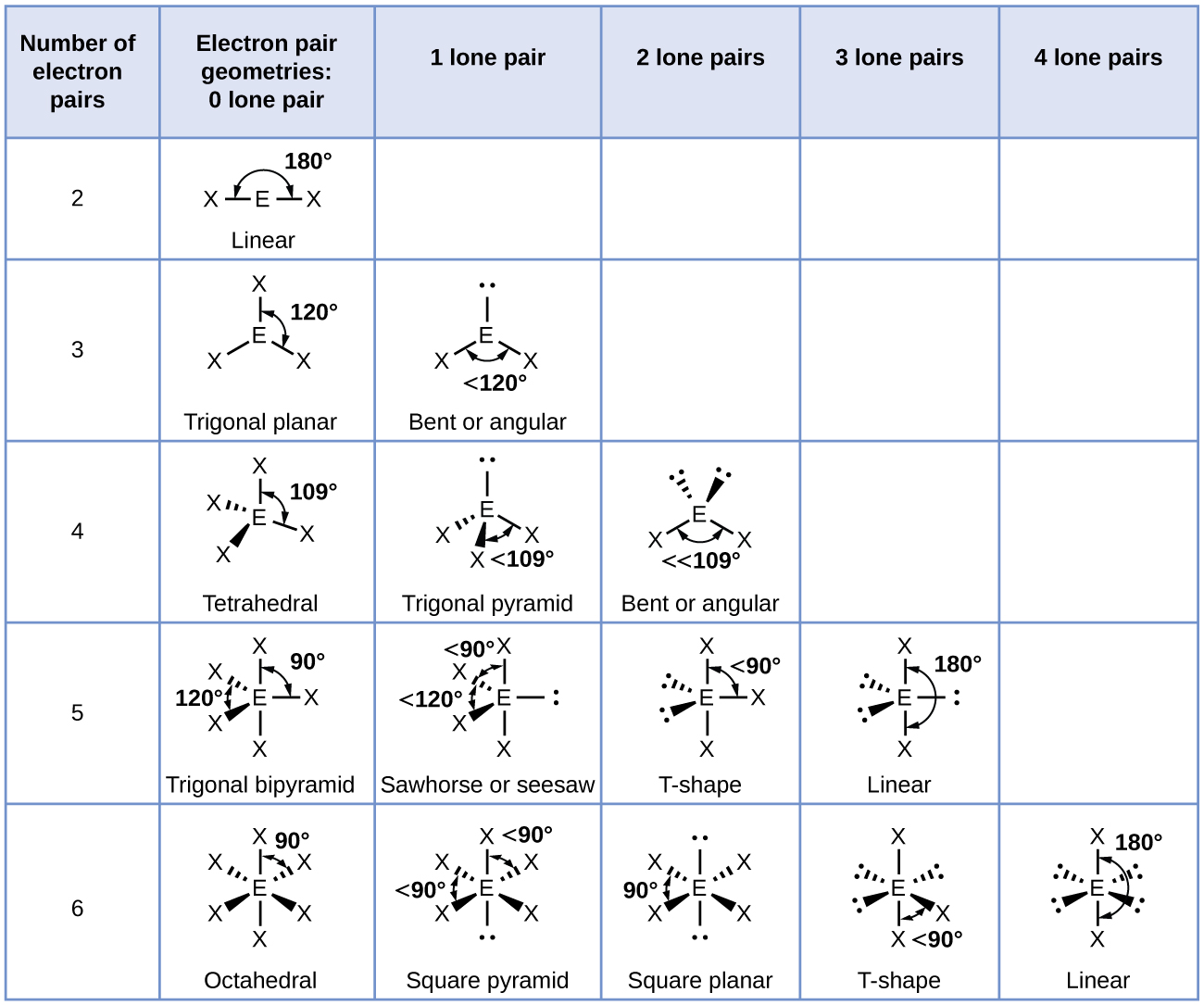
1. carbon dioxide, CO₂, a molecule produced by the combustion of fossil fuels

Solution

(a) We write the Lewis structure of CO₂ as:

This shows us two regions of high electron density around the carbon atom—each double bond counts as one region, and there are no lone pairs on the carbon atom. Using VSEPR theory, we predict that the two regions of electron density arrange themselves on opposite sides of the central atom with a bond angle of 180°. The electron-pair geometry and molecular structure are identical, and CO₂ molecules are linear.

Exercise \(\PageIndex{1}\)

Carbonate, \(\ce{CO3^2-}\), is a common polyatomic ion found in various materials from eggshells to antacids. What are the electron-pair geometry and molecular structure of this polyatomic ion?

Answer

The electron-pair geometry is trigonal planar and the molecular structure is trigonal planar. Due to resonance, all three C–O bonds are identical. Whether they are single, double, or an average of the two, each bond counts as one region of electron density.

Example \(\PageIndex{2}\): Predicting Electron-pair Geometry and Molecular Structure

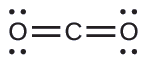
Two of the top 50 chemicals produced in the United States, ammonium nitrate and ammonium sulfate, both used as fertilizers, contain the ammonium ion. Predict the electron-pair geometry and molecular structure of the \(\ce{NH4+}\) cation.

Solution

We write the Lewis structure of \(\ce{NH4+}\) as:

Figure \(\PageIndex{7}\)).

Figure \(\PageIndex{8}\): The ammonium ion displays a tetrahedral electron-pair geometry as well as a tetrahedral molecular structure.

The next several examples illustrate the effect of lone pairs of electrons on molecular structure.

Example \(\PageIndex{3}\): Lone Pairs on the Central Atom

Predict the electron-pair geometry and molecular structure of a water molecule.

Solution

The Lewis structure of H₂O indicates that there are four regions of high electron density around the oxygen atom: two lone pairs and two chemical bonds:

Figure \(\PageIndex{9}\). Thus, the electron-pair geometry is tetrahedral and the molecular structure is bent with an angle slightly less than 109.5°. In fact, the bond angle is 104.5°.

Figure \(\PageIndex{9}\): (a) H₂O has four regions of electron density around the central atom, so it has a tetrahedral electron-pair geometry. (b) Two of the electron regions are lone pairs, so the molecular structure is bent.

Exercise \(\PageIndex{3}\)

The hydronium ion, H₃O⁺, forms when acids are dissolved in water. Predict the electron-pair geometry and molecular structure of this cation.

Answer

electron pair geometry: tetrahedral; molecular structure: trigonal pyramidal

Molecular Structure for Multicenter Molecules

When a molecule or polyatomic ion has only one central atom, the molecular structure completely describes the shape of the molecule. Larger molecules do not have a single central atom, but are connected by a chain of interior atoms that each possess a “local” geometry. The way these local structures are oriented with respect to each other also influences the molecular shape, but such considerations are largely beyond the scope of this introductory discussion. For our purposes, we will only focus on determining the local structures.

Example \(\PageIndex{5}\): Predicting Structure in Multicenter Molecules

The Lewis structure for the simplest amino acid, glycine, H₂NCH₂CO₂H, is shown here. Predict the local geometry for the nitrogen atom, the two carbon atoms, and the oxygen atom with a hydrogen atom attached:

Solution

Consider each central atom independently. The electron-pair geometries:

• nitrogen––four regions of electron density; tetrahedral
• carbon (CH₂)––four regions of electron density; tetrahedral
• carbon (CO₂)—three regions of electron density; trigonal planar
• oxygen (OH)—four regions of electron density; tetrahedral

The local structures:

• nitrogen––three bonds, one lone pair; trigonal pyramidal
• carbon (CH₂)—four bonds, no lone pairs; tetrahedral
• carbon (CO₂)—three bonds (double bond counts as one bond), no lone pairs; trigonal planar
• oxygen (OH)—two bonds, two lone pairs; bent (109°)

Exercise \(\PageIndex{5}\)

Another amino acid is alanine, which has the Lewis structure shown here. Predict the electron-pair geometry and local structure of the nitrogen atom, the three carbon atoms, and the oxygen atom with hydrogen attached:

Answer

electron-pair geometries: nitrogen––tetrahedral; carbon (CH)—tetrahedral; carbon (CH₃)—tetrahedral; carbon (CO₂)—trigonal planar; oxygen (OH)—tetrahedral; local structures: nitrogen—trigonal pyramidal; carbon (CH)—tetrahedral; carbon (CH₃)—tetrahedral; carbon (CO₂)—trigonal planar; oxygen (OH)—bent (109°)

Example \(\PageIndex{6}\): Molecular Simulation

Using this molecular shape simulator allows us to control whether bond angles and/or lone pairs are displayed by checking or unchecking the boxes under “Options” on the right. We can also use the “Name” checkboxes at bottom-left to display or hide the electron pair geometry (called “electron geometry” in the simulator) and/or molecular structure (called “molecular shape” in the simulator).

Build the molecule HCN in the simulator based on the following Lewis structure:

\(\mathrm{H–C≡N}\)

Click on each bond type or lone pair at right to add that group to the central atom. Once you have the complete molecule, rotate it to examine the predicted molecular structure. What molecular structure is this?

Solution

The molecular structure is linear.

Exercise \(\PageIndex{6}\)

Build a more complex molecule in the simulator. Identify the electron-group geometry, molecular structure, and bond angles. Then try to find a chemical formula that would match the structure you have drawn.

Answer

Answers will vary. For example, an atom with four single bonds, a double bond, and a lone pair has an octahedral electron-group geometry and a square pyramidal molecular structure. XeOF₄ is a molecule that adopts this structure.

Molecular Polarity and Dipole Moment

As discussed previously, polar covalent bonds connect two atoms with differing electronegativities, leaving one atom with a partial positive charge (δ+) and the other atom with a partial negative charge (δ–), as the electrons are pulled toward the more electronegative atom. This separation of charge gives rise to a bond dipole moment. The magnitude of a bond dipole moment is represented by the Greek letter mu (µ).

This bond moment can be represented as a vector, a quantity having both direction and magnitude (Figure \(\PageIndex{12}\)). Dipole vectors are shown as arrows pointing along the bond from the less electronegative atom toward the more electronegative atom. A small plus sign is drawn on the less electronegative end to indicate the partially positive end of the bond. The length of the arrow is proportional to the magnitude of the electronegativity difference between the two atoms.

Figure \(\PageIndex{12}\): (a) There is a small difference in electronegativity between C and H, represented as a short vector. (b) The electronegativity difference between B and F is much larger, so the vector representing the bond moment is much longer.

A whole molecule may also have a separation of charge, depending on its molecular structure and the polarity of each of its bonds. If such a charge separation exists, the molecule is said to be a polar molecule (or dipole); otherwise the molecule is said to be nonpolar. The dipole moment measures the extent of net charge separation in the molecule as a whole. We determine the dipole moment by adding the bond moments in three-dimensional space, taking into account the molecular structure.

For diatomic molecules, there is only one bond, so its bond dipole moment determines the molecular polarity. Homonuclear diatomic molecules such as Br₂ and N₂ have no difference in electronegativity, so their dipole moment is zero. For heteronuclear molecules such as CO, there is a small dipole moment. For HF, there is a larger dipole moment because there is a larger difference in electronegativity.

When a molecule contains more than one bond, the geometry must be taken into account. If the bonds in a molecule are arranged such that their bond moments cancel (vector sum equals zero), then the molecule is nonpolar. This is the situation in CO₂ (Figure \(\PageIndex{13A}\)). Each of the bonds is polar, but the molecule as a whole is nonpolar. From the Lewis structure, and using VSEPR theory, we determine that the CO₂ molecule is linear with polar C=O bonds on opposite sides of the carbon atom. The bond moments cancel because they are pointed in opposite directions. In the case of the water molecule (Figure \(\PageIndex{13B}\)), the Lewis structure again shows that there are two bonds to a central atom, and the electronegativity difference again shows that each of these bonds has a nonzero bond moment. In this case, however, the molecular structure is bent because of the lone pairs on O, and the two bond moments do not cancel. Therefore, water does have a net dipole moment and is a polar molecule (dipole).

Figure \(\PageIndex{13}\): The overall dipole moment of a molecule depends on the individual bond dipole moments and how they are arranged. (a) Each CO bond has a bond dipole moment, but they point in opposite directions so that the net CO₂ molecule is nonpolar. (b) In contrast, water is polar because the OH bond moments do not cancel out.

The OCS molecule has a structure similar to CO₂, but a sulfur atom has replaced one of the oxygen atoms. To determine if this molecule is polar, we draw the molecular structure. VSEPR theory predicts a linear molecule:

The C–O bond is considerably polar. Although C and S have very similar electronegativity values, S is slightly more electronegative than C, and so the C-S bond is just slightly polar. Because oxygen is more electronegative than sulfur, the oxygen end of the molecule is the negative end.

Chloromethane, CH₃Cl, is another example of a polar molecule. Although the polar C–Cl and C–H bonds are arranged in a tetrahedral geometry, the C–Cl bonds have a larger bond moment than the C–H bond, and the bond moments do not completely cancel each other. All of the dipoles have a upward component in the orientation shown, since carbon is more electronegative than hydrogen and less electronegative than chlorine:

When we examine the highly symmetrical molecules BF₃ (trigonal planar), CH₄ (tetrahedral), PF₅ (trigonal bipyramidal), and SF₆ (octahedral), in which all the polar bonds are identical, the molecules are nonpolar. The bonds in these molecules are arranged such that their dipoles cancel. However, just because a molecule contains identical bonds does not mean that the dipoles will always cancel. Many molecules that have identical bonds and lone pairs on the central atoms have bond dipoles that do not cancel. Examples include H₂S and NH₃. A hydrogen atom is at the positive end and a nitrogen or sulfur atom is at the negative end of the polar bonds in these molecules:

To summarize, to be polar, a molecule must:

1. Contain at least one polar covalent bond.
2. Have a molecular structure such that the sum of the vectors of each bond dipole moment does not cancel.

Properties of Polar Molecules

Polar molecules tend to align when placed in an electric field with the positive end of the molecule oriented toward the negative plate and the negative end toward the positive plate (Figure \(\PageIndex{14}\)). We can use an electrically charged object to attract polar molecules, but nonpolar molecules are not attracted. Also, polar solvents are better at dissolving polar substances, and nonpolar solvents are better at dissolving nonpolar substances.

Figure \(\PageIndex{14}\): (a) Molecules are always randomly distributed in the liquid state in the absence of an electric field. (b) When an electric field is applied, polar molecules like HF will align to the dipoles with the field direction.

Example \(\PageIndex{7}\): Polarity Simulations

Open the molecule polarity simulation and select the “Three Atoms” tab at the top. This should display a molecule ABC with three electronegativity adjustors. You can display or hide the bond moments, molecular dipoles, and partial charges at the right. Turning on the Electric Field will show whether the molecule moves when exposed to a field, similar to Figure \(\PageIndex{14}\).

Use the electronegativity controls to determine how the molecular dipole will look for the starting bent molecule if:

1. A and C are very electronegative and B is in the middle of the range.
2. A is very electronegative, and B and C are not.

Solution

1. Molecular dipole moment points immediately between A and C.
2. Molecular dipole moment points along the A–B bond, toward A.

Exercise \(\PageIndex{7}\)

Determine the partial charges that will give the largest possible bond dipoles.

Answer

The largest bond moments will occur with the largest partial charges. The two solutions above represent how unevenly the electrons are shared in the bond. The bond moments will be maximized when the electronegativity difference is greatest. The controls for A and C should be set to one extreme, and B should be set to the opposite extreme. Although the magnitude of the bond moment will not change based on whether B is the most electronegative or the least, the direction of the bond moment will.

Summary

VSEPR theory predicts the three-dimensional arrangement of atoms in a molecule. It states that valence electrons will assume an electron-pair geometry that minimizes repulsions between areas of high electron density (bonds and/or lone pairs). Molecular structure, which refers only to the placement of atoms in a molecule and not the electrons, is equivalent to electron-pair geometry only when there are no lone electron pairs around the central atom. A dipole moment measures a separation of charge. For one bond, the bond dipole moment is determined by the difference in electronegativity between the two atoms. For a molecule, the overall dipole moment is determined by both the individual bond moments and how these dipoles are arranged in the molecular structure. Polar molecules (those with an appreciable dipole moment) interact with electric fields, whereas nonpolar molecules do not.

Glossary

bond angle

angle between any two covalent bonds that share a common atom

bond distance

(also, bond length) distance between the nuclei of two bonded atoms

bond dipole moment

separation of charge in a bond that depends on the difference in electronegativity and the bond distance represented by partial charges or a vector

dipole moment

property of a molecule that describes the separation of charge determined by the sum of the individual bond moments based on the molecular structure

electron-pair geometry

arrangement around a central atom of all regions of electron density (bonds, lone pairs, or unpaired electrons)

linear

shape in which two outside groups are placed on opposite sides of a central atom

molecular structure

structure that includes only the placement of the atoms in the molecule

polar molecule

(also, dipole) molecule with an overall dipole moment

tetrahedral

shape in which four outside groups are placed around a central atom such that a three-dimensional shape is generated with four corners and 109.5° angles between each pair and the central atom

trigonal planar

shape in which three outside groups are placed in a flat triangle around a central atom with 120° angles between each pair and the central atom

valence shell electron-pair repulsion theory (VSEPR)

theory used to predict the bond angles in a molecule based on positioning regions of high electron density as far apart as possible to minimize electrostatic repulsion

vector

quantity having magnitude and direction

Contributors and Attributions

• Paul Flowers (University of North Carolina - Pembroke), Klaus Theopold (University of Delaware) and Richard Langley (Stephen F. Austin State University) with contributing authors. Textbook content produced by OpenStax College is licensed under a Creative Commons Attribution License 4.0 license. Download for free at http://cnx.org/contents/85abf193-2bd...a7ac8df6@9.110).