
9.2: Functions of Two Independent Variables
- Page ID
- 238249

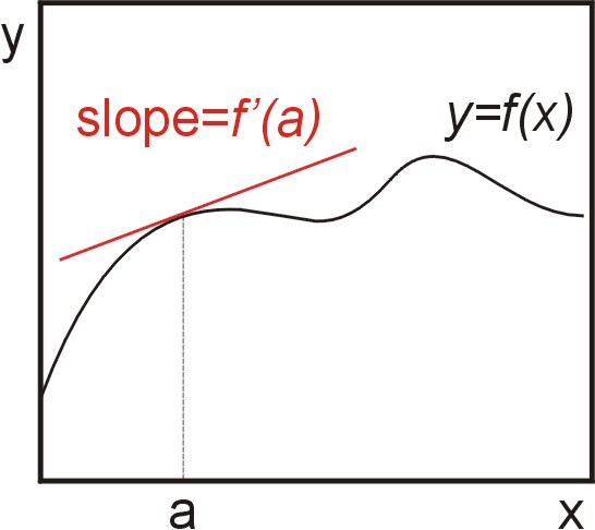
A (real) function of one variable, \(y = f(x)\), defines a curve in the plane. The first derivative of a function of one variable can be interpreted graphically as the slope of a tangent line, and dynamically as the rate of change of the function with respect to the variable Figure \(\PageIndex{1}\).
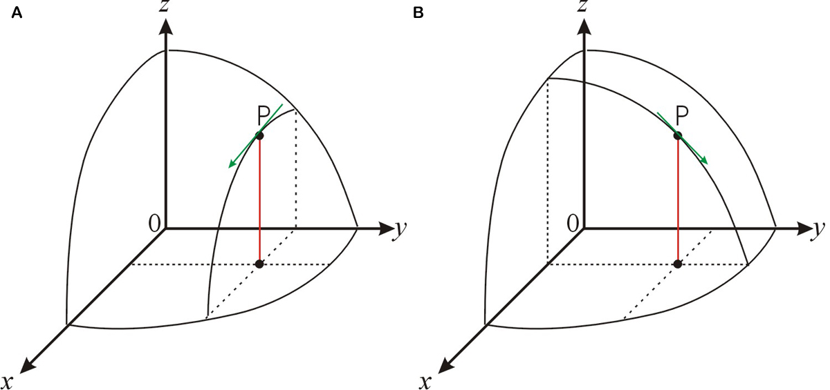
A function of two independent variables, \(z=f (x,y)\), defines a surface in three-dimensional space. For a function of two or more variables, there are as many independent first derivatives as there are independent variables. For example, we can differentiate the function \(z=f (x,y)\) with respect to \(x\) keeping \(y\) constant. This derivative represents the slope of the tangent line shown in Figure \(\PageIndex{2} \text{A}\). We can also take the derivative with respect to \(y\) keeping \(x\) constant, as shown in Figure \(\PageIndex{2} \text{B}\).
For example, let’s consider the function \(z=3x^2-y^2+2xy\). We can take the derivative of this function with respect to \(x\) treating \(y\) as a constant. The result is \(6x+2y\). This is the partial derivative of the function with respect to \(x\), and it is written:
\[\left (\frac{\partial z}{\partial x} \right )_y=6x+2y \nonumber\]
where the small subscripts indicate which variables are held constant. Analogously, the partial derivate of \(z\) with respect to \(y\) is:
\[\left (\frac{\partial z}{\partial y} \right )_x=2x-2y \nonumber\]
We can extend these ideas to functions of more than two variables. For example, consider the function \(f(x,y,z)=x^2y/z\). We can differentiate the function with respect to \(x\) keeping \(y\) and \(z\) constant to obtain:
\[\left (\frac{\partial f}{\partial x} \right )_{y,z}=2x\frac{y}{z} \nonumber\]
We can also differentiate the function with respect to \(z\) keeping \(x\) and \(y\) constant:
\[\left (\frac{\partial f}{\partial z} \right )_{x,y}=-x^2y/z^2 \nonumber\]
and differentiate the function with respect to \(y\) keeping \(x\) and \(z\) constant:
\[\left (\frac{\partial f}{\partial y} \right )_{x,z}=\frac{x^2}{z} \nonumber\]
Functions of two or more variables can be differentiated partially more than once with respect to either variable while holding the other constant to yield second and higher derivatives. For example, the function \(z=3x^2-y^2+2xy\) can be differentiated with respect to \(x\) two times to obtain:
\[\left ( \frac{\partial }{\partial x}\left ( \frac{\partial z}{\partial x} \right )_{y} \right )_{y}=\left ( \frac{\partial ^2z}{\partial x^2} \right )_{y}=6 \nonumber\]
We can also differentiate with respect to \(x\) first and \(y\) second:
\[\left ( \frac{\partial }{\partial y}\left ( \frac{\partial f}{\partial x} \right )_{y} \right )_{x}=\left ( \frac{\partial ^2f}{\partial y \partial x} \right )=2 \nonumber\]
Check the videos below if you are learning this for the first time, or if you feel you need to refresh the concept of partial derivatives.
- Partial derivatives: http://patrickjmt.com/derivatives-finding-partial-derivatives (don’t get confused by the different notation!)
- Partial derivatives: http://www.youtube.com/watch?v=vxJR5graUfI
- Higher order partial derivatives: http://www.youtube.com/watch?v=3itjTS2Y9oE
If a function of two or more variables and its derivatives are single-valued and continuous, a property normally attributed to physical variables, then the mixed partial second derivatives are equal (Euler reciprocity):
\[\label{c2v:euler reciprocity} \left ( \frac{\partial ^2f}{\partial x \partial y} \right )=\left ( \frac{\partial ^2f}{\partial y \partial x} \right )\]
For example, for \(z=3x^2-y^2+2xy\):
\[\left ( \frac{\partial ^2f}{\partial y \partial x} \right )=\left ( \frac{\partial }{\partial y}\left ( \frac{\partial f}{\partial x} \right )_{y} \right )_{x}=\left ( \frac{\partial }{\partial y}\left ( 6x+2y\right ) \right )_{x}=2 \nonumber\]
\[\left ( \frac{\partial ^2f}{\partial x \partial y} \right )=\left ( \frac{\partial }{\partial x}\left ( \frac{\partial f}{\partial y} \right )_{x} \right )_{y}=\left ( \frac{\partial }{\partial x}\left ( -2y+2x\right ) \right )_{y}=2 \nonumber\]
Another useful property of the partial derivatives is the so-called reciprocal identity, which holds when the same variables are held constant in the two derivatives:
\[\label{c2v:inverse} \left ( \frac{\partial y}{\partial x} \right )=\frac{1}{\left ( \frac{\partial x}{\partial y} \right )}\]
For example, for \(z=x^2y\):
\[\left ( \frac{\partial z}{\partial x} \right )_y=\left ( \frac{\partial }{\partial x} x^2y\right )_y=2xy \nonumber\]
\[\left ( \frac{\partial x}{\partial z} \right )_y=\left ( \frac{\partial }{\partial z} \sqrt{z/y} \right )_y=\frac{1}{2y} (z/y)^{-1/2}=\frac{1}{2xy}=\frac{1}{\left ( \frac{\partial z}{\partial x} \right )}_y \nonumber\]
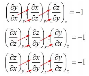
Finally, let’s mention the cycle rule. For a function \(z(x,y)\):
\[\label{c2v:cycle} \left ( \frac{\partial y}{\partial x} \right )_z\left ( \frac{\partial x}{\partial z} \right )_y\left ( \frac{\partial z}{\partial y} \right )_x=-1\]
We can construct other versions as follows:
For example, for \(z=x^2y\):
\[\left ( \frac{\partial y}{\partial x} \right )_z=\left ( \frac{\partial }{\partial x} (z/x^2)\right )_z=-2z/x^3 \nonumber\]
\[\left ( \frac{\partial x}{\partial z} \right )_y=\left ( \frac{\partial }{\partial z} \sqrt{z/y}\right )_y=\frac{1}{2y} (z/y)^{-1/2} \nonumber\]
\[\left ( \frac{\partial z}{\partial y} \right )_x=\left ( \frac{\partial }{\partial y} x^2y\right )_x=x^2 \nonumber\]
\[\left ( \frac{\partial y}{\partial x} \right )_z\left ( \frac{\partial x}{\partial z} \right )_y\left ( \frac{\partial z}{\partial y} \right )_x=-\frac{2z}{x^3}\frac{1}{2y} \left(\frac{y}{z}\right)^{1/2}x^2=-\left(\frac{z}{y}\right)^{1/2}\frac{1}{x}=-\left(\frac{x^2y}{y}\right)^{1/2}\frac{1}{x}=-1 \nonumber\]
Before discussing partial derivatives any further, let’s introduce a few physicochemical concepts to put our discussion in context.