7.2: Discrete Random Variables (2 of 5)

 

Learning Objectives

• Use probability distributions for discrete and continuous random variables to estimate probabilities and identify unusual events.

Probability Distribution for Discrete Random Variables

In this section, we work with probability distributions for discrete random variables. Here is an example:

Example

Consider the random variable the number of times a student changes major.

(For convenience, it is common practice to say: Let X be the random variable number of changes in major, or X = number of changes in major, so that from this point we can simply refer to X, with the understanding of what it represents.)

Here is the probability distribution of the random variable X:

Here is what it tells us:

For a randomly selected student, we cannot predict how many times he or she will change majors, but there is a predictable pattern described by the probability distribution (or model) above. So this is a random variable for which we are assuming the values range from 0 to 8. (In reality, a negligible proportion of students change majors more than 8 times.) The table provides a way to assign probabilities to outcomes. Note that if we add up the probabilities of all possible outcomes (0.135 + 0.271 + … + 0.002), we get exactly 1, which is not surprising (because one of the possible outcomes 0, 1, … , 8 will occur for sure).

Another way to represent the probability distribution of a random variable is with a probability histogram.

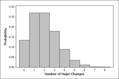
The horizontal axis accounts for the range of all possible values of the random variable (in our case, 0–8), and the vertical axis represents the probabilities of those values.

The heights of the bars add to 1, which is not surprising since the heights represent probabilities.

Let’s summarize the features of a probability distribution:

• The outcomes described by the model are random. This means that individual outcomes are uncertain, but there is a regular, predictable distribution of outcomes in a large number of repetitions.
• The model provides a way of assigning probabilities to all possible outcomes.
• The probability of each possible outcome can be viewed as the relative frequency of the outcome in a large number of repetitions, so like any other probability, it can be any value between 0 and 1.
• The sum of the probabilities of all possible outcomes must be 1.

Comment

Where do these probability distributions come from? Recall that probability distributions can come from data, such as the distribution of boreal owl eggs. Scientists observe thousands of nests and record the number of eggs in each nest. Then they calculate the relative frequency of each outcome. The relative frequency of each outcome represents the empirical probability for that outcome.

We can also use a mathematical formula to represent a probability distribution. In this case, we make assumptions about how outcomes will be distributed. In other words, we use a mathematical formula to describe the predicted relative frequencies for all possible outcomes. We do not look at mathematical formulas for probability distributions in this course, but we want you to be aware that not all probability distributions come from data.

Example

Recall the probability distribution of the random variable X = number of changes in major:

Let’s see what kinds of probability questions we can answer using it.

1. What is the probability that a college student will change majors at most once?

The phrase “at most once” means either the student never changes majors (X = 0) or the student changes majors once (X = 1). Therefore, to find this probability, we need to add the probabilities that are highlighted in the table:

So,

P(a college student changes majors at most once) = P(X = 0) + P(X = 1) = 0.135 + 0.271 = 0.406

The probability that a randomly selected college student will change majors at most once is about 0.406. We can also say that about 40.6% of the time, a randomly selected college student will change majors at most once.

2. John’s parents are concerned that he has decided to change his major for the second time. John claims that he is not unusual. What is the probability that a randomly selected college student will change his major as often as or more often than John?

To answer the question about John, we need know the probability that a randomly selected student will change his major 2 or more times. We need to add together the probabilities shaded in the table.

P(change major 2 or more times) = P(X = 2) + P(X = 3) + … + P(X = 8) = 0.594

Here is another way to figure this out. We can use the idea that all of the probabilities together make up 100% of the possibilities. So if we add up all the probabilities in the table we should get 1. Now if we figure out the probability that someone changes majors 0 or 1 times, we can just subtract this from 1 to find the probability that someone changes majors 2 or more times. As we learned previously, this is the complement rule.

P(change major 2 or more times) = 1 – [P(X = 0) + P(X = 1)] = 1 – [0.135 + 0.271] = 0.594

Do you think John has given a convincing argument that he is not unusual? Yes! Fifty-nine percent of the time, a college student will change majors as often as or more often than John did. Stating this same result in terms of probability, we might say, “There is a 59% probability that a randomly selected college student will change majors 2 or more times while in college.”

Learn By Doing

https://assessments.lumenlearning.co...sessments/3875

Learn By Doing

https://assessments.lumenlearning.co...sessments/3876

We found that changing a major 2 or more times is not very unusual, since it happens about 59% of the time. So…

3. How often would John need to change his major to be considered unusual?

One way to answer this question is to just a make a judgment call about what we might consider “unusual” based on the table. For example, we might notice that the probability that a student will change majors 5 or more times is about 5%.

P(change majors 5 or more times)	= P(X = 5) + P(X = 6) + P(X = 7) + P(X = 8)
	= 0.036 + 0.012 + 0.003 + 0.002 = 0.053

An event that occurs only 5% of the time is pretty unusual.

Are there other ways to more definitively determine what might be considered unusual? Well, we might use a measure of center, such as the mean, to determine a “typical” number of times that students change majors. Values that are 2 standard deviations above the mean could be used to identify unusual behavior. We will come back to this question after we have developed an understanding of mean and standard deviation for a probability distribution.

 

CC licensed content, Shared previously

• Concepts in Statistics. Provided by: Open Learning Initiative. Located at: http://oli.cmu.edu. License: CC BY: Attribution