3.4: Mean and Median (1 of 2)

Last updated
Save as PDF

Page ID: 251291

$ \newcommand{\vecs}[1]{\overset { \scriptstyle \rightharpoonup} {\mathbf{#1}} } $ $ \newcommand{\vecd}[1]{\overset{-\!-\!\rightharpoonup}{\vphantom{a}\smash {#1}}} $$\newcommand{\id}{\mathrm{id}}$ $ \newcommand{\Span}{\mathrm{span}}$ $ \newcommand{\kernel}{\mathrm{null}\,}$ $ \newcommand{\range}{\mathrm{range}\,}$ $ \newcommand{\RealPart}{\mathrm{Re}}$ $ \newcommand{\ImaginaryPart}{\mathrm{Im}}$ $ \newcommand{\Argument}{\mathrm{Arg}}$ $ \newcommand{\norm}[1]{\| #1 \|}$ $ \newcommand{\inner}[2]{\langle #1, #2 \rangle}$ $ \newcommand{\Span}{\mathrm{span}}$ $\newcommand{\id}{\mathrm{id}}$ $ \newcommand{\Span}{\mathrm{span}}$ $ \newcommand{\kernel}{\mathrm{null}\,}$ $ \newcommand{\range}{\mathrm{range}\,}$ $ \newcommand{\RealPart}{\mathrm{Re}}$ $ \newcommand{\ImaginaryPart}{\mathrm{Im}}$ $ \newcommand{\Argument}{\mathrm{Arg}}$ $ \newcommand{\norm}[1]{\| #1 \|}$ $ \newcommand{\inner}[2]{\langle #1, #2 \rangle}$ $ \newcommand{\Span}{\mathrm{span}}$$\newcommand{\AA}{\unicode[.8,0]{x212B}}$

Learning Objectives

Use mean and median to describe the center of a distribution.

Recall that when we describe the distribution of a quantitative variable, we describe the overall pattern (shape, center, and spread) in the data and deviations from the pattern (outliers). In our previous discussion of patterns in quantitative data, we identified a typical value in the distribution. We used this single value of the variable to represent the entire group. This is an informal way to think about the center of the distribution. In “Measures of Center,” we focus on describing the center of a distribution more precisely.

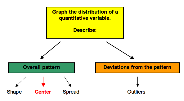
Flow chart that focuses on the center of an overall pattern.

We develop two different measurements for identifying the center of a distribution: the mean and the median. Each measure has special properties.

Mean

The mean is the average. It is written as $\stackrel{¯}{x}$ and pronounced “x-bar.” To calculate the mean, we add the data values and divide by the number of data points.

We can write this as a formula.

$\stackrel{¯}{x}=\frac{\mathrm{Σ}x}{n}$

In this formula, the symbol $\mathrm{Σ}$ means sum (add up the values). The x represents the data values. The letter “n” represents the number of data values.

Example

Calculating the Mean

Let’s find the mean of a set of three quiz scores: 70, 85, 82. In this situation, n is 3 because there are 3 quiz scores. We add the “x” values, 70 + 85 + 82 to get 237, then divide by 3 to get a mean of 79.

We could write this calculation using the formula:

$\stackrel{¯}{x}=\frac{\mathrm{Σ}x}{n}=\frac{70+85+82}{3}=\frac{237}{3}=79$

Example

Average Homework Score

Suppose Beth’s homework scores are70, 80, 80, 80, 85, 86, 90, 90, 95. There is variability in her homework scores, but the mean represents her typical performance on homework.

The mean of her scores is

$\stackrel{¯}{x}=\frac{70+80+80+80+85+86+90+90+95\text{}}{9}\text{}=\text{}\frac{756}{9}=84$

So Beth’s performance on homework varies, but on average, she makes an 84 on each assignment. In other words, we can understand the mean as the score Beth would have on every assignment if she always made the same grade – that is, if she made an 84 on all nine homework assignments.

Her mean score is 84, since

$\stackrel{¯}{x}=\frac{84+84+84+84+84+84+84+84+84\text{}}{9}\text{}=\text{}\frac{9(84)}{9}\text{}=\frac{756}{9}=84$

From this viewpoint, the mean is the fair share measure of center.

Notice, however, that Beth did not actually make an 84 on any assignment. The mean does not give us information about any individual homework score or about how the homework scores vary. It only gives us a sense of her performance by averaging the values across all the assignments.

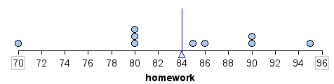
Here is the mean marked on a dotplot of the distribution of homework scores. For this set of scores, the mean appears to be a pretty good measure of how Beth performed overall.

Dotplot of the distribution of homework scores. The mean is eighty four percent.

The mean is also referred to as the balancing point of a distribution. If we measure the distance between each data point and the mean, the distances are balanced on each side of the mean.

For example, a homework score of 95 is 11 points above the mean, as shown.

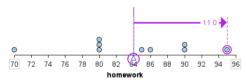
Dotplot where homework score of 95 is highlighted to show that it is eleven points above the mean.

A homework score of 80 is 4 points below the mean. In the table, we calculate the sum of the distances above and below the mean. Notice that the sum of the distances above and below the mean are equal. In this way, the mean is a balancing point for the distribution.

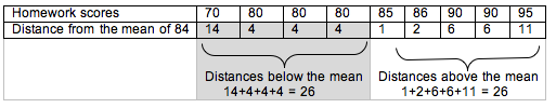
Table showing the sum of the distances above and below the mean

We can also view the distances below the mean as negative and the distances above the mean as positive. When we add these “signed” distances together, we get 0

(−14) + (−4) + (−4) + (−4) + 1 + 2 + 6 + 6 + 11

(−26) + 26

The mean is the only measure of center with this special property.

Median

The median is another way to identify a typical value. The median is the middle of the data when all the values are listed in order. The median divides the data into two equal-sized groups. There is as much data below the median as above it.

Example

Median Homework Score

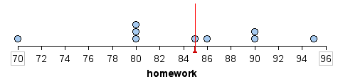
Let’s return to Beth’s homework scores: 70, 80, 80, 80, 85, 86, 90, 90, 95.

The median score is 85. This is the center score. There are four homework scores below 85 and four homework scores above 85.

For this data set, the median was one of the homework scores. This will not always be the case. So, like the mean, the median does not give us information about any individual homework score or about how the homework scores vary. It only gives us a sense of Beth’s performance by locating a value that is the middle of the actual scores.

Here is the median marked on a dotplot of the distribution of homework scores. For this set of scores, the median is also a pretty good measure of how Beth performed overall.

Dotplot showing the median of the distribution of homework scores, which is 85. The highest distribution is in the eightieth percentile

Learn By Doing

https://assessments.lumenlearning.co...sessments/3441

https://assessments.lumenlearning.co...sessments/3442

Concepts in Statistics. Provided by: Open Learning Initiative. Located at: http://oli.cmu.edu. License: CC BY: Attribution