
11.1: Reading- Profits and Losses with the Average Cost Curve
- Page ID
- 249380
Profits and Losses with the Average Cost Curve
Does maximizing profit (producing where MR = MC) imply an actual economic profit? The answer depends on the relationship between price and average total cost. If the price that a firm charges is higher than its average cost of production for that quantity produced, then the firm will earn profits. Conversely, if the price that a firm charges is lower than its average cost of production, the firm will suffer losses. You might think that, in this situation, the farmer may want to shut down immediately. Remember, however, that the firm has already paid for fixed costs, such as equipment, so it may continue to produce and incur a loss. Figure 8.5 illustrates three situations: (a) where price intersects marginal cost at a level above the average cost curve, (b) where price intersects marginal cost at a level equal to the average cost curve, and (c) where price intersects marginal cost at a level below the average cost curve.
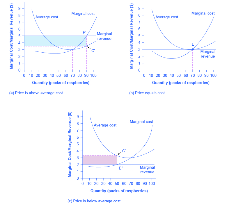
First consider a situation where the price is equal to $5 for a pack of frozen raspberries. The rule for a profit-maximizing perfectly competitive firm is to produce the level of output where Price = MR = MC, so the raspberry farmer will produce a quantity of 90, which is labeled as E in Figure 8.5 (a). Remember that the area of a rectangle is equal to its base multiplied by its height. The farm’s total revenue at this price will be shown by the larger rectangle starting from the origin right to a quantity of 90 packs (the base) up to point E (the height), left to the price of $5, and back down to the origin. The average cost of producing 90 packs is shown by point C or about $3.50. Total costs will be the quantity of 90 times the average cost of $3.50, which is shown by the area of the rectangle from the origin to a quantity of 90, up to point C, over to the vertical axis and down to the origin. It should be clear from examining the two rectangles that total revenue is greater than total cost. Thus, profits will be the blue shaded rectangle on top.
It can be calculated as:
| profit | = | total revenue − total cost |
| = | (90)($5.00) − (90)($3.50) | |
| = | $135 |
Or, it can be calculated as:
| profit | = | (price − average cost) × quantity |
| = | ($5.00 − $3.50) × 90 | |
| = | 135 |
Now consider Figure 8.5 (b), where the price has fallen to $3.00 for a pack of frozen raspberries. Again, the perfectly competitive firm will choose the level of output where Price = MR = MC, but in this case, the quantity produced will be 70. At this price and output level, where the marginal cost curve is crossing the average cost curve, the price received by the firm is exactly equal to its average cost of production.
The farm’s total revenue at this price will be shown by the large rectangle from the origin over to a quantity of 70 packs (the base) up to point E’ (the height), over to the price of $3, and back to the origin. The average cost of producing 70 packs is the same as the farm’s total revenue because the price of one unit is equal to the cost to produce that unit. Thus, the firm is making zero profit. The calculations are as follows:
| profit | = | total revenue − total cost |
| = | (70)($3.00) − (70)($3.00) | |
| = | $0 |
Or, it can be calculated as:
| profit | = | (price − average cost) × quantity |
| = | ($3.00 − $3.00) × 70 | |
| = | $0 |
In Figure 8.5 (c), the market price has fallen still further to $2.00 for a pack of frozen raspberries. At this price, marginal revenue intersects marginal cost at a quantity of 50. The farm’s total revenue at this price will be shown by the rectangle from the origin over to a quantity of 50 packs (the base) up to point E” (the height), over to the price of $2, and back to the origin. The average cost of producing 50 packs is shown by point C” or about $3.30. Total costs will be the quantity of 50 times the average cost of $3.30, which is shown by the area of the rectangle from the origin to a quantity of 50, up to point C”, over to the vertical axis and down to the origin. It should be clear from examining the two rectangles that total revenue is less than total cost. Thus, the firm is losing money and the loss (or negative profit) will be the rose-shaded rectangle.
The calculations are:
| profit | = | total revenue − total cost |
| = | (50)($2.00) − (50)($3.30) | |
| = | -$65.00 |
Or:
| profit | = | (price − average cost) × quantity |
| = | ($1.75 − $3.30) × 50 | |
| = | -$65.00 |
If the market price received by a perfectly competitive firm leads it to produce at a quantity where the price is greater than average cost, the firm will earn profits. If the price received by the firm causes it to produce at a quantity where price equals average cost, which occurs at the minimum point of the AC curve, then the firm earns zero profits. Finally, if the price received by the firm leads it to produce at a quantity where the price is less than average cost, the firm will earn losses. This is summarized in Table 8.4.
| Table 8.4 | ||
|---|---|---|
| If… | Then… | |
| Price > ATC | Firm earns an economic profit | |
| Price = ATC | Firm earns zero economic profit | |
| Price < ATC | Firm earns a loss | |
Watch this video to see the concept of economic profit explained:

A YouTube element has been excluded from this version of the text. You can view it online here: http://pb.libretexts.org/micro2/?p=360
Self Check: Profit and Losses in Competitive Markets
Answer the question(s) below to see how well you understand the topics covered in the previous section. This short quiz does not count toward your grade in the class, and you can retake it an unlimited number of times.
You’ll have more success on the Self Check if you’ve completed the Reading in this section.
Use this quiz to check your understanding and decide whether to (1) study the previous section further or (2) move on to the next section.
- Principles of Microeconomics Chapter 8.2. Authored by: OpenStax College. Provided by: Rice University. Located at: http://cnx.org/contents/6i8iXmBj@10.31:9ACVqdAi@13/How-Perfectly-Competitive-Firm. License: CC BY: Attribution. License Terms: Download for free at http://cnx.org/content/col11627/latest
- Perfect competition: Economic profit. Authored by: lostmy1. Provided by: University of South Africa. Located at: https://www.youtube.com/watch?v=qo9GQIcgOHI&index=5&list=PL616B7E47EF9203CC. License: CC BY: Attribution