10.7: Reading- Short Run and Long Run Average Total Costs

Last updated
Save as PDF

Page ID: 249365

\( \newcommand{\vecs}[1]{\overset { \scriptstyle \rightharpoonup} {\mathbf{#1}} } \) \( \newcommand{\vecd}[1]{\overset{-\!-\!\rightharpoonup}{\vphantom{a}\smash {#1}}} \)\(\newcommand{\id}{\mathrm{id}}\) \( \newcommand{\Span}{\mathrm{span}}\) \( \newcommand{\kernel}{\mathrm{null}\,}\) \( \newcommand{\range}{\mathrm{range}\,}\) \( \newcommand{\RealPart}{\mathrm{Re}}\) \( \newcommand{\ImaginaryPart}{\mathrm{Im}}\) \( \newcommand{\Argument}{\mathrm{Arg}}\) \( \newcommand{\norm}[1]{\| #1 \|}\) \( \newcommand{\inner}[2]{\langle #1, #2 \rangle}\) \( \newcommand{\Span}{\mathrm{span}}\) \(\newcommand{\id}{\mathrm{id}}\) \( \newcommand{\Span}{\mathrm{span}}\) \( \newcommand{\kernel}{\mathrm{null}\,}\) \( \newcommand{\range}{\mathrm{range}\,}\) \( \newcommand{\RealPart}{\mathrm{Re}}\) \( \newcommand{\ImaginaryPart}{\mathrm{Im}}\) \( \newcommand{\Argument}{\mathrm{Arg}}\) \( \newcommand{\norm}[1]{\| #1 \|}\) \( \newcommand{\inner}[2]{\langle #1, #2 \rangle}\) \( \newcommand{\Span}{\mathrm{span}}\)\(\newcommand{\AA}{\unicode[.8,0]{x212B}}\)

Short Run and Long Run Average Total Costs

As in the short run, costs in the long run depend on the firm’s level of output, the costs of factors, and the quantities of factors needed for each level of output. The chief difference between long- and short-run costs is there are no fixed factors in the long run. There are thus no fixed costs. All costs are variable, so we do not distinguish between total variable cost and total cost in the long run: total cost is total variable cost.

The long-run average cost (LRAC) curve shows the firm’s lowest cost per unit at each level of output, assuming that all factors of production are variable. The LRAC curve assumes that the firm has chosen the optimal factor mix, as described in the previous section, for producing any level of output. The costs it shows are therefore the lowest costs possible for each level of output. It is important to note, however, that this does not mean that the minimum points of each short-run ATC curves lie on the LRAC curve. This critical point is explained in the next paragraph and expanded upon even further in the next section.

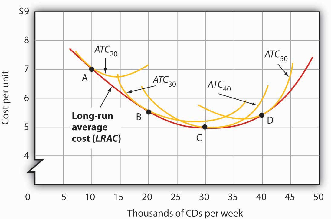
Figure 8.9 “Relationship Between Short-Run and Long-Run Average Total Costs” shows how a firm’s LRAC curve is derived. Suppose Lifetime Disc Co. produces compact discs (CDs) using capital and labor. We have already seen how a firm’s average total cost curve can be drawn in the short run for a given quantity of a particular factor of production, such as capital. In the short run, Lifetime Disc might be limited to operating with a given amount of capital; it would face one of the short-run average total cost curves shown in Figure 8.9 “Relationship Between Short-Run and Long-Run Average Total Costs.” If it has 30 units of capital, for example, its average total cost curve is ATC₃₀. In the long run the firm can examine the average total cost curves associated with varying levels of capital.

Four possible short-run average total cost curves for Lifetime Disc are shown in Figure 8.9 “Relationship Between Short-Run and Long-Run Average Total Costs” for quantities of capital of 20, 30, 40, and 50 units. The relevant curves are labeled ATC₂₀, ATC₃₀, ATC₄₀, and ATC₅₀ respectively. The LRAC curve is derived from this set of short-run curves by finding the lowest average total cost associated with each level of output. Again, notice that the U-shaped LRAC curve is an envelope curve that surrounds the various short-run ATC curves. With the exception of ATC₄₀, in this example, the lowest cost per unit for a particular level of output in the long run is not the minimum point of the relevant short-run curve.

Graph of the long-run average cost curve, which is rounded like a boat, and the smaller average total costs curves, which appear like small boats within the LRAC.

Figure 8.9 Relationship Between Short-Run and Long-Run Average Total Costs. The LRAC curve is found by taking the lowest average total cost curve at each level of output. Here, average total cost curves for quantities of capital of 20, 30, 40, and 50 units are shown for the Lifetime Disc Co. At a production level of 10,000 CDs per week, Lifetime minimizes its cost per CD by producing with 20 units of capital (point A). At 20,000 CDs per week, an expansion to a plant size associated with 30 units of capital minimizes cost per unit (point B). The lowest cost per unit is achieved with production of 30,000 CDs per week using 40 units of capital (point C). If Lifetime chooses to produce 40,000 CDs per week, it will do so most cheaply with 50 units of capital (point D).

Self Check: The Short Run vs. The Long Run

Answer the question(s) below to see how well you understand the topics covered in the previous section. This short quiz does not count toward your grade in the class, and you can retake it an unlimited number of times.

You’ll have more success on the Self Check if you’ve completed the two Readings in this section.

Use this quiz to check your understanding and decide whether to (1) study the previous section further or (2) move on to the next section.

https://assessments.lumenlearning.com/assessments/764

Principles of Microeconomics Section 8.2 . Authored by: Anonymous. Located at: http://2012books.lardbucket.org/books/microeconomics-principles-v2.0/s11-02-production-choices-and-costs-t.html. License: CC BY-NC-SA: Attribution-NonCommercial-ShareAlike