6.1: Why It Matters- Relationships in Categorical Data with Intro to Probability

Last updated
Save as PDF

Page ID: 251347

\( \newcommand{\vecs}[1]{\overset { \scriptstyle \rightharpoonup} {\mathbf{#1}} } \) \( \newcommand{\vecd}[1]{\overset{-\!-\!\rightharpoonup}{\vphantom{a}\smash {#1}}} \)\(\newcommand{\id}{\mathrm{id}}\) \( \newcommand{\Span}{\mathrm{span}}\) \( \newcommand{\kernel}{\mathrm{null}\,}\) \( \newcommand{\range}{\mathrm{range}\,}\) \( \newcommand{\RealPart}{\mathrm{Re}}\) \( \newcommand{\ImaginaryPart}{\mathrm{Im}}\) \( \newcommand{\Argument}{\mathrm{Arg}}\) \( \newcommand{\norm}[1]{\| #1 \|}\) \( \newcommand{\inner}[2]{\langle #1, #2 \rangle}\) \( \newcommand{\Span}{\mathrm{span}}\) \(\newcommand{\id}{\mathrm{id}}\) \( \newcommand{\Span}{\mathrm{span}}\) \( \newcommand{\kernel}{\mathrm{null}\,}\) \( \newcommand{\range}{\mathrm{range}\,}\) \( \newcommand{\RealPart}{\mathrm{Re}}\) \( \newcommand{\ImaginaryPart}{\mathrm{Im}}\) \( \newcommand{\Argument}{\mathrm{Arg}}\) \( \newcommand{\norm}[1]{\| #1 \|}\) \( \newcommand{\inner}[2]{\langle #1, #2 \rangle}\) \( \newcommand{\Span}{\mathrm{span}}\)\(\newcommand{\AA}{\unicode[.8,0]{x212B}}\)

Before we begin Relationships in Categorical Data with Intro to Probability, it is helpful to consider how it relates to the work we have already done in previous modules.

At the start of Summarizing Data Graphically and Numerically, we stated the difference between quantitative and categorical variables:

Quantitative variables have numeric values that can be averaged. A quantitative variable is frequently a measurement – for example, a person’s height in inches.
Categorical variables are variables that can have one of a limited number of values, or labels. Values that can be represented by categorical variables include, for example, a person’s eye color, gender, or home state; a vehicle’s body style (sedan, SUV, minivan, etc.); a dog’s breed (bulldog, greyhound, beagle, etc.).

The remainder of Summarizing Data Graphically and Numerically focused on describing the overall pattern (shape, center, and spread) of the distribution of a quantitative variable.

In and Examining Relationships: Quantitative Data and Nonlinear Models, our goal was to identify and model the relationship between two quantitative variables.

Now, in this module, we turn our full attention back to categorical variables. Our objective is to study the relationship between two categorical variables. Just as in Examining Relationships: Quantitative Data and Nonlinear Models, we will be looking for patterns in the data.

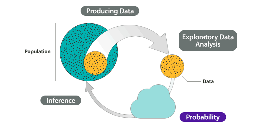
As we organize and analyze data from two categorical variables, we make extensive use of two-way tables. Two-way tables for two categorical variables are in some ways like scatterplots for two quantitative variables: they give us a useful snapshot of all of the data organized in terms of the two variables of interest. This will be helpful in finding and comparing patterns. This part of Relationships in Categorical Data with Intro to Probability is exploratory data analysis in the Big Picture of Statistics.

A second important objective of this module is to introduce you to the concept of probability. Two-way tables give us a practical context for talking about probability. We also use two-way tables to help us visualize and solve real-world problems involving probability. This part of the module is part of probability in the Big Picture of Statistics.

The Big Picture of Statistics. Shown on the diagram are Step 1: Producing Data, Step 2: Exploratory Data Analysis, Step 3: Probability, and Step 4: Inference. Highlighted in this diagram is Step 3: Probability

Concepts in Statistics. Provided by: Open Learning Initiative. Located at: http://oli.cmu.edu. License: CC BY: Attribution