11.6: Orbital Angular Momentum and the p-orbitals

Learning Objectives

• To relate the classical orbital angular momentum for an particle to the quantum equivalent
• Characterize the mangnitude and orientation of orbital angular momentum for an electron in terms of quantum numbers

Classical Orbital Angular Momentum

The physical quantity known as angular momentum plays a dominant role in the understanding of the electronic structure of atoms. To gain a physical picture and feeling for the angular momentum it is necessary to consider a model system from the classical point of view. The simplest classical model of the hydrogen atom is one in which the electron moves in a circular orbit with a constant speed or angular velocity (Figure 6.6.1 ). Just as the linear momentum \(m\vec{v}\) plays a dominant role in the analysis of linear motion, so angular momentum (\(L\)) plays the central role in the analysis of a system with circular motion as found in the model of the hydrogen atom.

Figure 6.6.1 : The angular momentum vector for a classical model of the atom. (CC BY-NC; Ümit Kaya via LibreTexts)

In Figure 6.6.1 , \(m\) is the mass of the electron, \(\vec{v}\) is the linear velocity (the velocity the electron would possess if it continued moving at a tangent to the orbit) and \(r\) is the radius of the orbit. The linear velocity \(\vec{v}\) is a vector since it possesses at any instant both a magnitude and a direction in space. Obviously, as the electron rotates in the orbit the direction of \(\vec{v}\) is constantly changing, and thus the linear momentum \(m\vec{v}\) is not constant for the circular motion. This is so even though the speed of the electron (i.e, the magnitude of \(\vec{v}\) which is denoted by \(|\vec{v}|\)) remains unchanged. According to Newton's second law, a force must be acting on the electron if its momentum changes with time. This is the force which prevents the electron from flying on tangent to its orbit. In an atom the attractive force which contains the electron is the electrostatic force of attraction between the nucleus and the electron, directed along the radius r at right angles to the direction of the electron's motion.

The angular momentum, like the linear momentum, is a vector and is defined as follows:

\[|\vec{L}| = m \nu r \nonumber \]

The angular momentum vector \(\vec{L}\) is directed along the axis of rotation. From the definition it is evident that the angular momentum vector will remain constant as long as the speed of the electron in the orbit is constant (\(|\vec{v}|\) remains unchanged) and the plane and radius of the orbit remain unchanged. Thus for a given orbit, the angular momentum is constant as long as the angular velocity of the particle in the orbit is constant. In an atom the only force on the electron in the orbit is directed along \(r\); it has no component in the direction of the motion. The force acts in such a way as to change only the linear momentum. Therefore, while the linear momentum is not constant during the circular motion, the angular momentum is. A force exerted on the particle in the direction of the vector \(\vec{v}\) would change the angular velocity and the angular momentum. When a force is applied which does change \(\vec{L}\), a torque is said to be acting on the system. Thus angular momentum and torque are related in the same way as are linear momentum and force.

Quantum Angular Momentum

The important point of the above discussion is that both the angular momentum and the energy of an atom remain constant if the atom is left undisturbed. Any physical quantity which is constant in a classical system is both conserved and quantized in a quantum mechanical system. Thus both the energy and the angular momentum are quantized for an atom.

Any physical quantity which is constant in a classical system is both conserved and quantized in a quantum mechanical system.

There is a quantum number, denoted by \(l\), which governs the magnitude of the angular momentum, just as the quantum number \(n\) determines the energy. The magnitude of the angular momentum may assume only those values given by:

\[ |L| = \sqrt{l(l+1)} \hbar \label{4} \]

with \(l = 0, 1, 2, 3, ... n-1\).

Furthermore, the value of n limits the maximum value of the angular momentum as the value of l cannot be greater than n - 1. For the state n = 1 discussed above, \(l\) may have the value of zero only. When n = 2, l may equal 0 or 1, and for n = 3, l = 0 or 1 or 2, etc. When l = 0, it is evident from Equation \(\ref{4}\) that the angular momentum of the electron is zero. The atomic orbitals which describe these states of zero angular momentum are called s orbitals. The s orbitals are distinguished from one another by stating the value of n, the principal quantum number. They are referred to as the 1s, 2s, 3s, etc., atomic orbitals.

The preceding discussion referred to the 1s orbital since for the ground state of the hydrogen atom \(n = 1\) and \(l = 0\). This orbital, and all s orbitals in general, predict spherical density distributions for the electron as discussed previously.

It is common usage to refer to an electron as being "in" an orbital even though an orbital is, but a mathematical function with no physical reality. To say an electron is in a particular orbital is meant to imply that the electron is in the quantum state which is described by that orbital. For example, when the electron is in the 2s orbital the hydrogen atom is in a state for which \(n = 2\) and \(l = 0\).

Comparing these results with those for the 1s orbital in Figure 6.6.2 we see that as \(n\) increases the average value of \(r\) increases. This agrees with the fact that the energy of the electron also increases as \(n\) increases. The increased energy results in the electron being on the average pulled further away from the attractive force of the nucleus. As in the simple example of an electron moving on a line, nodes (values of \(r\) for which the electron density is zero) appear in the probability distributions. The number of nodes increases with increasing energy and equals \(n - 1\).

When the electron possesses angular momentum the density distributions are no longer spherical. In fact for each value of \(l\), the electron density distribution assumes a characteristic shapes in Figure 6.6.2 .

Figure 6.6.2 : The appearance of the three 2p orbitals in three-dimensional space. (CC BY-SA 3.0; I, Sarxos).

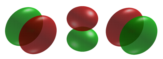
When \(l = 1\), the orbitals are called p orbitals. In this case the orbital and its electron density are concentrated along a line (axis) in space. The 2p orbital or wavefunction is positive in value on one side and negative in value on the other side of a plane which is perpendicular to the axis of the orbital and passes through the nucleus. The orbital has a node in this plane, and consequently an electron in a 2p orbital does not place any electronic charge density at the nucleus. The electron density of a 1s orbital, on the other hand, is a maximum at the nucleus. The same diagram for the 2p density distribution is obtained for any plane which contains this axis. Thus in three dimensions the electron density would appear to be concentrated in two lobes, one on each side of the nucleus, each lobe being circular in cross section Figure 6.6.3 .

An electron possesses orbital angular momentum has a density distributions is no longer spherical.

The \(m_l\) Quantum Number and Magnetic Fields

The magnetic quantum number, designated by the letter \(m_l\), is the third quantum numbers which describe the unique quantum state of an electron. The magnetic quantum number distinguishes the orbitals available within a subshell, and is used to calculate the azimuthal component of the orientation of the orbital in space. As with our discussion of rigid rotors, the quantum number \(m_l\) refers to the projection of the angular momentum in this arbitrarily chosen direction, conventionally called the \(z\) direction or quantization axis. \(L_z\), the magnitude of the angular momentum in the z direction, is given by the formula

\[ L_z = m_l \hbar \nonumber \]

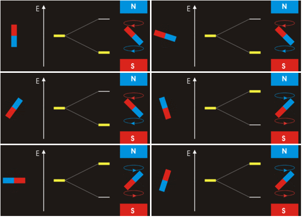
The quantum number \(m_l\) refers, loosely, to the direction of the angular momentum vector. The magnetic quantum number \(m_l\) only affects the electron's energy if it is in a magnetic field because in the absence of one, all spherical harmonics corresponding to the different arbitrary values of \(m_l\) are equivalent. The magnetic quantum number determines the energy shift of an atomic orbital due to an external magnetic field (this is called the Zeeman effect) - hence the name magnetic quantum number. However, the actual magnetic dipole moment of an electron in an atomic orbital arrives not only from the electron angular momentum, but also from the electron spin, expressed in the spin quantum number, which is the fourth quantum number. \(m_s\) and discussed in the next chapter.

Figure 6.6.3 : The orbiting electron with a non-zero \(l\) value acts like a magnetic field with is no energetic difference for any particular orientation (only one energy state, on the left). However, in external magnetic field there is a high-energy state and a low-energy state depending on the relative orientations of the magnet to the external field. (CC SA-BY 3.0; Darekk2).

Which \(m_l\) Number Corresponds to which p-Orbital?

The answer is complicated; while \(m_l=0\) corresponds to the \(p_z\), the orbitals for \(m_l=+1\) and \(m_l=−1\) lie in the xy-plane (see Spherical Harmonics), but not on the axes. The reason for this outcome is that the wavefunctions are usually formulated in spherical coordinates to make the math easier, but graphs in the Cartesian coordinates make more intuitive sense for humans. The \(p_x\) and \(p_y\) orbitals are constructed via a linear combination approach from radial and angular wavefunctions and converted into \(xy\) (this was discussed previously). Thus, it is not possible to directly correlate the values of \(m_l=±1\) with specific orbitals. The notion that we can do so is sometimes presented in introductory courses to make a complex mathematical model just a little bit simpler and more intuitive, but it is incorrect.

The three wavefunctions for \(n=2\) and \(l=1\) are as follows.

\[ \begin{align} |\psi_{2,1,0} \rangle &=r \cos θR(r) \\[4pt] |\psi_{2,1,+1} \rangle &=−\dfrac{r}{2} \sinθ e^{iϕ} R(r) \\[4pt] |\psi_{2,1,-1} \rangle &=+\dfrac{r}{2} \sinθ e^{-iϕ} R(r) \end{align} \nonumber \]

The notation is \(|\psi_{n,l,m_l} \rangle\) with \(R(r)\) is the radial component of this wavefuction, \(θ\) is the angle with respect to the z-axis and \(ϕ\) is the angle with respect to the \(xz\)-plane.

\[R(r)=\sqrt{\dfrac{Z^5}{32\pi a_0^5}}\mathrm{e}^{-Zr/2a_0} \nonumber \]

in which \(Z\) is the atomic number (or probably better nuclear charge) and \(a_0\) is the Bohr radius.

In switching from spherical to Cartesian coordinates, we make the substitution \(z=r \cosθ\), so:

\[|\psi_{2,1,0} \rangle =z R(r) \nonumber \]

This is \(\psi_{2p_z}\) since the value of \(\psi \) is dependent on \(z\): when \(z=0\); \(\psi =0\), which is expected since \(z=0\) describes the \(xy\)-plane.

The other two wavefunctions are degenerate in the \(xy\)-plane. An equivalent statement is that these two orbitals do not lie on the x- and y-axes, but rather bisect them. Thus it is typical to take linear combinations of them to make the equation look prettier. If any set of wavefunctions is a solution to the Schrödinger equation, then any set of linear combinations of these wavefunctions must also be a solution (Section 2.4). We can do this because of the linearity of the Schrödinger equation.

In the equations below, we're going to make use of some trigonometry, notably Euler's formula:

\[ \begin{align} \mathrm{e}^{\mathrm{i}\phi} &=\cos{\phi}+\mathrm{i}\sin{\phi}\\[4pt] \sin{\phi} &= \dfrac{\mathrm{e}^{\mathrm{i}\phi}-\mathrm{e}^{-\mathrm{i}\phi}}{2\mathrm{i}}\\[4pt] \cos{\phi} &= \dfrac{\mathrm{e}^{\mathrm{i}\phi}+\mathrm{e}^{-\mathrm{i}\phi}}{2} \end{align} \nonumber \]

We're also going to use \(x=\sin θ\cos ϕ\) and \(y=\sin θ \sinϕ \).

\begin{align*} \psi_{2p_x} &=\dfrac{1}{\sqrt{2}}\left(\psi_{2,1,+1}-\psi_{2,1,-1}\right) \\[4pt] &=\dfrac{1}{2}\left(\mathrm{e}^{\mathrm{i}\phi}+\mathrm{e}^{-\mathrm{i}\phi} \right)r\sin{\theta} f(r) \\[4pt] &=r\sin{\theta}\cos{\phi}f(r)=xf(r) \\[4pt] \psi_{2p_y} &=\dfrac{\mathrm{i}}{\sqrt{2}}\left(\psi_{2,1,+1}+\psi_{2,1,-1}\right)\\[4pt] &=\dfrac{1}{2\mathrm{i}}\left(\mathrm{e}^{\mathrm{i}\phi}-\mathrm{e}^{-\mathrm{i}\phi} \right)r\sin{\theta}f(r)\\[4pt] &=r\sin{\theta}\sin{\phi}f(r)=yf(r)\\ \end{align*}

So, while \(m_l=0\) corresponds to \(|p_z \rangle\), \(m_l=+1\) and \(m_l=−1\) cannot be directly assigned to either \(|p_x \rangle\) or \(|p_y \rangle\), but rather a combination of \(|p_x \rangle\) and \(|p_y \rangle\). An alternative description is that \(m_l=+1\) might correspond to \((|p_x \rangle\ + |p_y \rangle )\) and \(m_l=−1\) might correspond to \((|p_x \rangle\ - |p_y \rangle)\).

d-Orbitals (even higher angular momenta wavefunctions)

When \(l = 2\), the orbitals are called d orbitals and Figure 6.6.4 shows the contours in a plane for a 3d orbital and its density distribution. Notice that the density is again zero at the nucleus and that there are now two nodes in the orbital and in its density distribution. As the angular momentum of the electron increases, the density distribution becomes increasingly concentrated along an axis or in a plane in space. Only electrons in \(s\) orbitals with zero angular momentum give spherical density distributions and in addition place charge density at the position of the nucleus.

Figure 6.6.4 : The appearance of the 3d electron density distribution in three-dimensional space. (CC BY-SA 3.0; I, Sarxos)

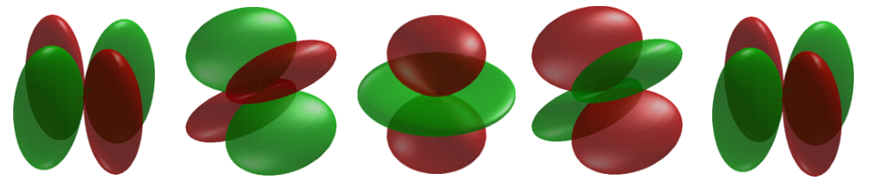
As with the p-orbitals, the only d-orbital that a specific \(m_l\) can be ascribed is the \(d_{z^2}\) orbitals with \(m_l=0\). The rest are linear combinations of the hydrogen atom wavefunctions with complex spherical harmonic angular components.

There seems to be neither rhyme nor reason for the naming of the states corresponding to the different values of \(\ell\) (s, p, d, f for l = 0, 1, 2, 3). This set of labels had its origin in the early work of experimental atomic spectroscopy. The letter s stood for sharp, p for principal, d for diffuse and f for fundamental in characterizing spectral lines. From the letter f onwards the naming of the orbitals is alphabetical \(l = 4,5,6 \rightarrow g,h,i, ....\).

We have not as yet accounted for the full degeneracy of the hydrogen atom orbitals which we stated earlier to be \(n^2\) for every value of \(n\). For example, when \(n = 2\), there are four distinct atomic orbitals. The remaining degeneracy is again determined by the angular momentum of the system. Since angular momentum like linear momentum is a vector quantity, we may refer to the component of the angular momentum vector which lies along some chosen axis. For reasons we shall investigate, the number of values a particular component can assume for a given value of \(l\) is (\(2l + 1\)). Thus when \(l = 0\), there is no angular momentum and there is but a single orbital, an s orbital. When \(l = 1\), there are three possible values for the component (\(2 \times 1 + 1\)) of the total angular momentum which are physically distinguishable from one another. There are, therefore, three p orbitals. Similarly there are five d orbitals, (\(2 \times 2+1\)), seven f orbitals, (\(2 \times 3 +1\)), etc. All of the orbitals with the same value of \(n\) and \(l\), the three 2p orbitals for example, are similar but differ in their spatial orientations.

To gain a better understanding of this final element of degeneracy, we must consider in more detail what quantum mechanics predicts concerning the angular momentum of an electron in an atom.

Contributors and Attributions

• David M. Hanson, Erica Harvey, Robert Sweeney, Theresa Julia Zielinski ("Quantum States of Atoms and Molecules")

• Dr. Richard F.W. Bader  (Professor of Chemistry / McMaster University)

• Stack Exchange (Ben Norris and Loong)