3.5.6: BF₃

The case of boron trifluoride (\(\ce{BF_3}\)) is an example of a molecule with one more layer of complexity than the other examples we have seen in previous sections in this chapter. (\(\ce{BF_3}\)) is more complex than previous examples because it is the first case in which there are multiple types of valence orbitals on the pendant atoms. (\(\ce{BF_3}\)) possesses \(s\) and \(p\) orbitals on both the central atom and all of the pendant atoms. We can follow the same steps that we have previously to derive other molecular orbital diagrams; however, there is one important difference: we will treat each type of pendant orbital as an individual set of SALCs.

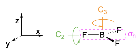
Step 1. Find the point group of the molecule and assign Cartesian coordinates so that z is the principal axis.

The BH\(_3\) molecule is trigonal planar, and its point group is \(D_{3h}\). The \(z\) axis is colinear with the principle axis, the \(C_3\) axis.

Figure \(\PageIndex{1}\): The molecule is in the \(D_{3h}\) point group. (CC-BY-NC-SA; Kathryn Haas)

Step 2. Identify and count the pendant atoms' valence orbitals.

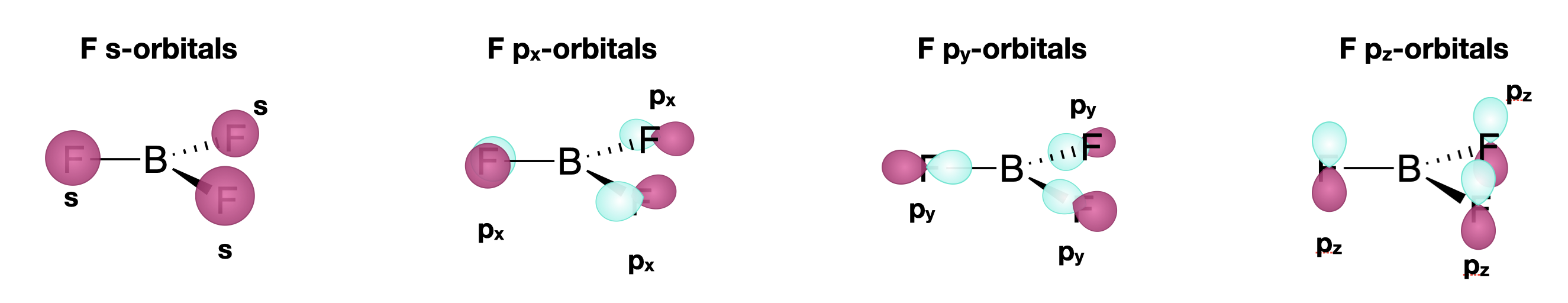
Each of the three pendant fluorine atoms has four valence orbitals: one \(2s\) and three \(2p\) orbitals. Thus, we can expect a total of twelve SALCs from the three atoms. However, we will treat each type of orbital from the F atoms as its own set; each will have its own set of coordinates, with the \(y\) axis along the M-L bond. Thus we expect the following:

• One set of \(2s\) SALCs: there is one 2s orbital on each of three atoms. This set will have three SALCs.
• One set of \(2p_x\) SALCs: there is one \(2p_x\) orbital on each of three atoms. Each of these individual orbitals is perpendicular to the M-L bond and coplanar with the molecule. This set will have three SALCs.
• One set of \(2p_y\) SALCs: there is one \(2p_y\) orbital on each of three atoms. Each of these individual orbitals is colinear with the M-L bond. This set will have three SALCs.
• One set of \(2p_z\) SALCs: there is one \(2p_z\) orbital on each of three atoms. Each of these individual orbitals is perpendicular to the M-L bond and parallel with the principal axis of the molecule. This set will have three SALCs.

Figure \(\PageIndex{2}\): Individual sets of pendant fluorine atomic orbitals will create separate sets of SALCs. (CC-BY-SA; Kathryn Haas)

Step 3. Generate the \(\Gamma\)'s for each set of SALCs

Use the \(D_{3h}\) character table to generate one reducible representation (\(\Gamma\)) for each of the four sets of pendant atomic orbitals shown in Figure \(\PageIndex{2}\); in this case we need four \(\Gamma\) because there are four types of valence orbital (the \(s, p_x, p_y, p_z\)).

• For the set of \(s\) orbitals: perform the operation for each class in the character table. Each \(s\) orbital is assigned a value depending on whether it moves or not: assign a value of 1 if it remains in place during the operation, or 0 (zero) if it moves out of its original place.
• for each set of \(p\) orbitals: Now there are phases (signs of the wavefunction), so a negative value is possible. Assign a value of 1 to each \(p\) orbital if it remains in place and in phase during the operation; assign a -1 if the atom's position remains, while the phase of the orbital is inverted (the positive lobe moves to the position of the negative lobe and vice versa); assign a 0 if it moves out of its original position.

The \(\Gamma\) for each type is given below:
\[\begin{array}{|c|cccccc|} \hline \bf{D_{3h}} & E & 2C_3 & 3C_2 & \sigma_h & 2S_3 & 3\sigma_v \\ \hline
\bf{\Gamma_{2s}} & 3 & 0 & 1 & 3 & 0 & 1 \\
\bf{\Gamma_{2p_x}} & 3 & 0 & -1 & 3 & 0 & -1 \\
\bf{\Gamma_{2p_y}} & 3 & 0 & 1 & 3 & 0 & 1 \\
\bf{\Gamma_{2p_z}} & 3 & 0 & -1 & -3 & 0 & 1 \\
\hline \end{array} \nonumber \]

Step 4. Break \(\Gamma\)'s into irreducible representations for individual SALCs

Reduce each \(\Gamma\) into its component irreducible representations. Using either of the processes described previously, we find that each of the \(\Gamma\) reduces to two irreducible representations under the \(D_{3h}\) point group; in each case one is singly degenerate (\(A\)) and the other doubly degenerate (\(E\)). This equates to three SALCs for each \(\Gamma\) (orbital type) and a total of twelve SALCs. This should give us confidence! We were in fact expecting 12 SALCs because we found that there were twelve pendant atomic orbitals to start with.

\[\begin{array}{|c|cccccc|} \hline {D_{3h}} & E & 2C_3 & 3C_2 & \sigma_h & 2S_3 & 3\sigma_v \\ \hline
\bf{\Gamma_{2s}} & \bf 3 & \bf 0 & \bf 1 & \bf 3 & \bf 0 & \bf 1 \\
A_{1}' & 1 & 1 & 1 & 1 & 1 & 1 \\
E' & 2 & -1 & 0 & 2 & -1 & 0 \\
\hline \end{array} \nonumber \]

\[\begin{array}{|c|cccccc|} \hline {D_{3h}} & E & 2C_3 & 3C_2 & \sigma_h & 2S_3 & 3\sigma_v \\ \hline
\bf{\Gamma_{2p_x}} &\bf 3 &\bf 0 &\bf -1 &\bf 3 &\bf 0 &\bf -1 \\
A_{2}' & 1 & 1 & -1 & 1 & 1 & -1 \\
E' & 2 & -1 & 0 & 2 & -1 & 0 \\
\hline \end{array} \nonumber \]

\[\begin{array}{|c|cccccc|} \hline {D_{3h}} & E & 2C_3 & 3C_2 & \sigma_h & 2S_3 & 3\sigma_v \\ \hline
\bf{\Gamma_{2p_y}} &\bf 3 &\bf 0 &\bf 1 &\bf 3 &\bf 0 &\bf 1 \\
A_{1}' & 1 & 1 & 1 & 1 & 1 & 1 \\
E' & 2 & -1 & 0 & 2 & -1 & 0 \\
\hline \end{array} \nonumber \]

\[\begin{array}{|c|cccccc|} \hline {D_{3h}} & E & 2C_3 & 3C_2 & \sigma_h & 2S_3 & 3\sigma_v \\ \hline
\bf{\Gamma_{2p_z}} &\bf 3 &\bf 0 &\bf -1 &\bf -3 &\bf 0 &\bf 1 \\
A_{2}" & 1 & 1 & -1 & -1 & -1 & 1 \\
E" & 2 & -1 & 0 & -2 & 1 & 0 \\
\hline \end{array} \nonumber \]

Step 5: Sketch the SALCs

We'll skip this step for now to make this problem simpler.

Step 6: Draw the MO diagram by combining SALCs with AO’s of like symmetry.

We now know the symmetries of different pendant orbital SALCs - and it is helpful if we also know their relative energies, and the energies of the valence orbitals on the central boron atom. We can make predictions based on periodic trends, or we can use a table of ionization energies as a guide. The symmetries of the boron \(2s\) and \(2p\) orbitals can be found from the \(D_{3h}\) character table.