3.5.2: Carbon Dioxide

Construct SALCs and the molecular orbital diagram for CO\(_2\).

Carbon dioxide is another linear molecule. This example is slightly more complex than the previous example of the bifluoride anion. While bifluoride had only one valence orbital to consider in its central H atom (the \(1s\) orbital), carbon dioxide has a larger central atom, and thus more valence orbitals that will interact with SALCs.

Preliminary Steps

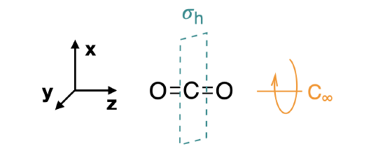
Step 1. Find the point group of the molecule and assign Cartesian coordinates so that z is the principal axis.

The CO\(_2\) molecule is linear and its point group is \(D_{\infty h}\). The \(z\) axis is collinear with the \(C_\infty\) axis. We will use the \(D_{2h}\) point group as a substitute since the orbital symmetries are retained in the \(D_{2h}\) point group.

Figure \(\PageIndex{1}\): CO\(_2\) belongs to the \(D_{\infty h}\) point group. (CC_BY-NC-SA; Kathryn Haas)

Step 2. Identify and count the pendant atoms' valence orbitals.

Each of the two pendant oxygen atoms has four valence orbitals; \(2s\), \(2p_x\), \(2p_y\), and \(2p_z\). Thus, we can expect a total of eight SALCs.

Generate SALCs

The SALCs for CO\(_2\) are identical in shape and symmetry to those described in the previous example for the bifluoride anion. But instead of cutting to the shortcut, we will systematically derive the SALCs here to demonstrate the process.

Step 3. Generate the \(\Gamma\)'s

Use the \(D_{2h}\) character table to generate four reducible representations (\(\Gamma's\)); one for each of the four types of pendant atom orbitals (\(s, \;p_x, \;p_y, \;p_z\)). For each \(s\) orbital, assign a value of 1 if it remains in place during the operation or zero if it moves out of its original place. For each \(p\) orbital, assign 1 if there is no change, -1 if it remains in place but is inverted, and 0 if it moves out of its original position. The four \(\Gamma\)'s are given below:
\[\begin{array}{|c|cccccccc|} \hline \bf{D_{2h}} & E & C_2(z) & C_2(y) &C_2(x) & i &\sigma(xy) & \sigma(xz) & \sigma(yz)\\ \hline \bf{\Gamma_{2s}} & 2 & 2 & 0 & 0 & 0 & 0 & 2 & 2 \\ \bf{\Gamma_{2p_x}} & 2 & -2 & 0 & 0 & 0 & 0 & 2 & -2 \\ \bf{\Gamma_{2p_y}} & 2 & -2 & 0 & 0 & 0 & 0 & -2 & 2 \\ \bf{\Gamma_{2p_z}} & 2 & 2 & 0 & 0 & 0 & 0 & 2 & 2 \\ \hline \end{array} \nonumber \]

Step 4. Break \(\Gamma\)'s into irreducible representations for individual SALCs

Reduce each \(\Gamma\) into its component irreducible representations. There are two strategies that can be used to do this. The quick and easy way is to do it "by inspection", but this only works well for simple cases. The other is by using the systematic approach for breaking a \(\Gamma\) into reducible representations described previously in section 4.4.2 using the following formula:
\[\text{# of } i = \frac{1}{h}\sum(\text{# of operations in class)}\times(\chi_{\Gamma}) \times (\chi_i) \label{irs} \]
In other words, the number of irreducible representations of type \(i\) is equal to the sum of the number of operations in the class \(\times\) the character of the \(\Gamma_{modes}\) \(\times\) the character of \(i\), and that sum is divided by the order of the group (\(h\)).

Using either approach results in the following eight irreducible representations (\(2A_{g} + 2B_{1u} + B_{2g} + B_{3u} + B_{3g} + B_{2u}\)):

\[\begin{array}{|c|c|cccccccc|} \hline \bf{D_{2h}} & E & C_2(z) & C_2(y) &C_2(x) & i &\sigma(xy) & \sigma(xz) & \sigma(yz)\\ \hline
\bf{\Gamma_{2s} = A_g + B_{1u}} &\bf{\Gamma_{2s}} & \bf{2} & \bf{2} & \bf{0} & \bf{0} & \bf{0} & \bf{0} & \bf{2} & \bf{2}\\
& A_{g} & 1 & 1 & 1 & 1 & 1 & 1 & 1 & 1 \\
& B_{1u} & 1 & 1 & -1 & -1 & -1 & -1 & 1 & 1 \\
\hline \\ \hline

\bf{\Gamma_{2p_x} = B_{2g} + B_{3u}} &\bf{\Gamma_{2p_x}} & \bf{2} & \bf{-2} & \bf{0} & \bf{0} & \bf{0} & \bf{0} & \bf{2} & \bf{-2} \\
& B_{2g} & 1 & -1 & 1 & -1 & 1 & -1 & 1 & -1 \\
& B_{3u} & 1 & -1 & -1 & 1 & -1 & 1 & 1 & -1 \\
\hline \\ \hline

\bf{\Gamma_{2p_y}=B_{3g}+B_{2u}} & \bf{\Gamma_{2p_y}} & \bf2 & \bf-2 & \bf0 & \bf0 & \bf0 & \bf0 & \bf-2 & \bf2 \\
& B_{3g} & 1 & -1 & -1 & 1 & 1 & -1 & -1 & 1 \\
& B_{2u} & 1 & -1 & 1 & -1 & -1 & 1 & -1 & 1 \\
\hline \\ \hline

\bf{\Gamma_{2p_z} = A_{g}+B_{1u}} & \bf{\Gamma_{2p_z}} & \bf{2} & \bf{2} & \bf{0} & \bf{0} & \bf{0} & \bf{0} & \bf{2} & \bf{2}\\
& A_{g} & 1 & 1 & 1 & 1 & 1 & 1 & 1 & 1 \\
& B_{1u} & 1 & 1 & -1 & -1 & -1 & -1 & 1 & 1 \\ \hline \end{array} \nonumber \]

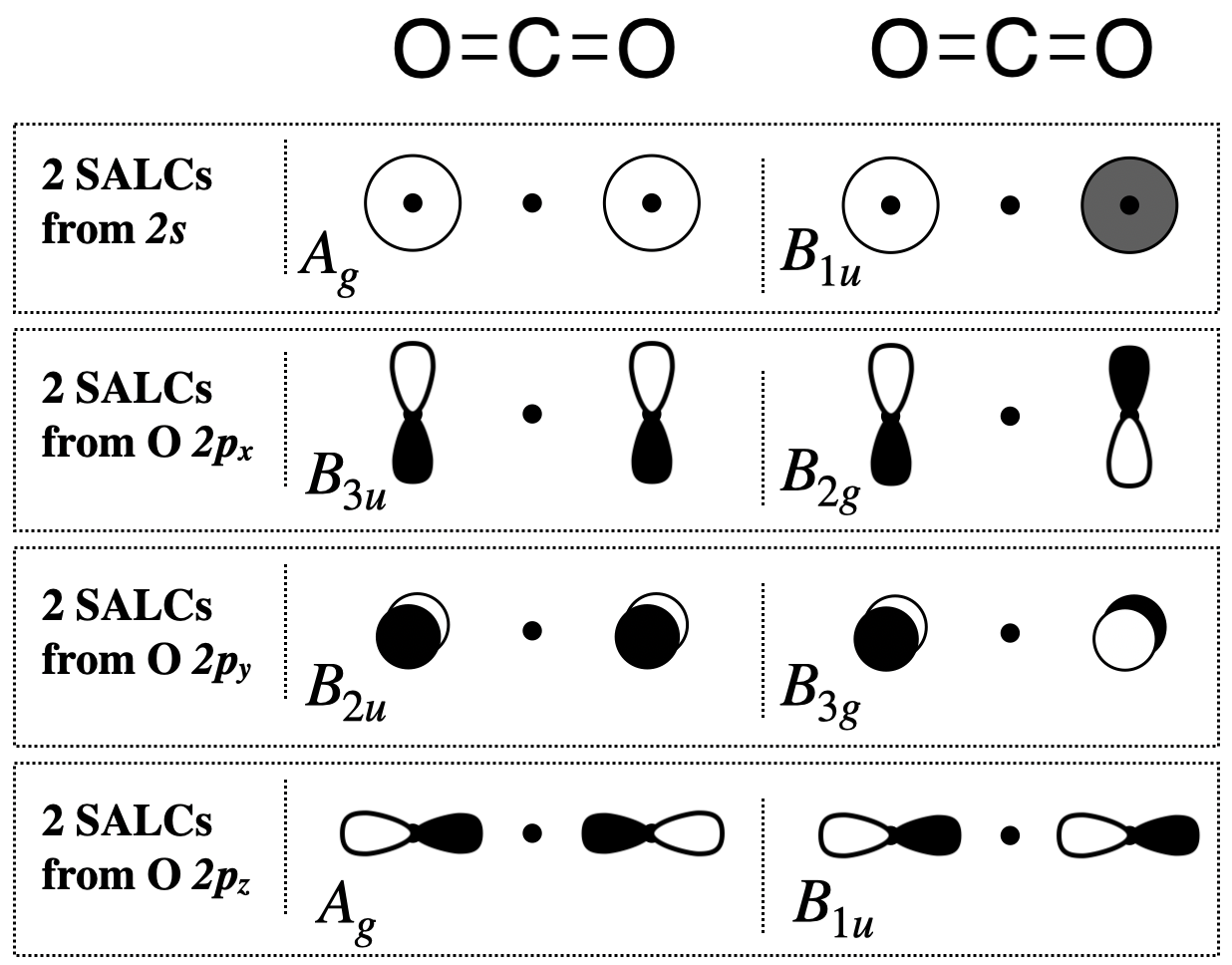
Step 5. Sketch the SALCs

From the systematic process above, you have found the symmetries (the irreducible representations) of all eight SALCs under the \(D_{2h}\) point group. To sketch the SALC that corresponds to each irreducible representation, again we use the \(D_{2h}\) character table, and specifically the functions listed on the right side columns of the table.

Two \(A_g\) SALCs (one from \(s\) and one from \(p_z\)): The \(A_g\) SALCs are each singly degenerate and symmetric with respect to both the principal axis (\(z\)) and the inversion center (\(i\)) (based on its Mulliken Label). We can look at the functions in the \(D_{2h}\) character table that correspond to \(A_g\) and see that it is completely symmetric under the group (because the combination of \(x^2,y^2,z^2\) shows that it is totally symmetric). This would be the same symmetry as an \(s\) orbital on the central atom. From this information, we know that these SALCs must have symmetry compatible with an \(s\) orbital on the central atom, and we can draw the two \(A_g\) SALCs shown in Figure \(\PageIndex{2}\).

Two \(B_{1u}\) SALCs (one from \(s\) and one from \(p_z\)): The Mulliken Label tells us that the \(B_{1u}\) SALCs are each antisymmetric with respect to both the principal axis and the inversion center. The function, \(z\), appearing with \(B_{1u}\) in the character table tells us that these SALCs have the same symmetry as the \(z\) axis, or a \(p_z\) orbital on the central atom. From this information, we know that these two SALCs should be compatible with a \(p_z\) orbital on the central atom, and we can draw the two \(B_{1u}\) SALCs shown in Figure \(\PageIndex{2}\).

All other SALCs shown below are derived using a strategy similar to the one in the two cases described above.

Figure \(\PageIndex{2}\): SALCs from the valence orbitals of oxygen atoms in CO\(_2\). (CC-BY-NC-SA; Kathryn Haas)

Draw the MO diagram for \(CO_2\)

Step 6. Combine SALCs with AO’s of like symmetry.

First we identify the valence orbitals on carbon: there are four including \(2s\), \(2p_x\), \(2p_y\), and \(2p_z\). Now we identify the symmetry of each using the \(D_{2h}\) character table. The symmetry of a central \(s\) orbital corresponds to the combination of functions \(x^2\), \(y^2\), and \(z^2\) in the character table; this is \(A_g\). The \(p_z\) orbital corresponds to the symmetry of the linear function \(z\) in the character table; this is \(B_{1u}\). And so on... The symmetries of the C valence orbitals are listed below. \[2s =A_g \\ 2p_x = B_{3u} \\ 2p_y = B_{2u} \\ 2p_z = B_{1u} \nonumber \]

Now that we have identified the symmetries of the eight oxygen SALCs and the four valence orbitals on carbon, we know which atomic orbitals and SALCs may combine based on compatible symmetries. We also need to know the relative orbital energy levels so that we can predict the relative strength of orbital interactions. The orbital ionization energies are listed in Section 5.3.

With knowledge of both orbital symmetries and energies, we can construct the molecular orbital diagram. The carbon atom goes on one side of the diagram while the oxygen SALCs are drawn on the opposite side. Molecular orbitals are drawn in the center column of the diagram:

Figure \(\PageIndex{3}\): Molecular orbital diagram for carbon dioxide. (CC-BY-NC-SA; Kathryn Haas)

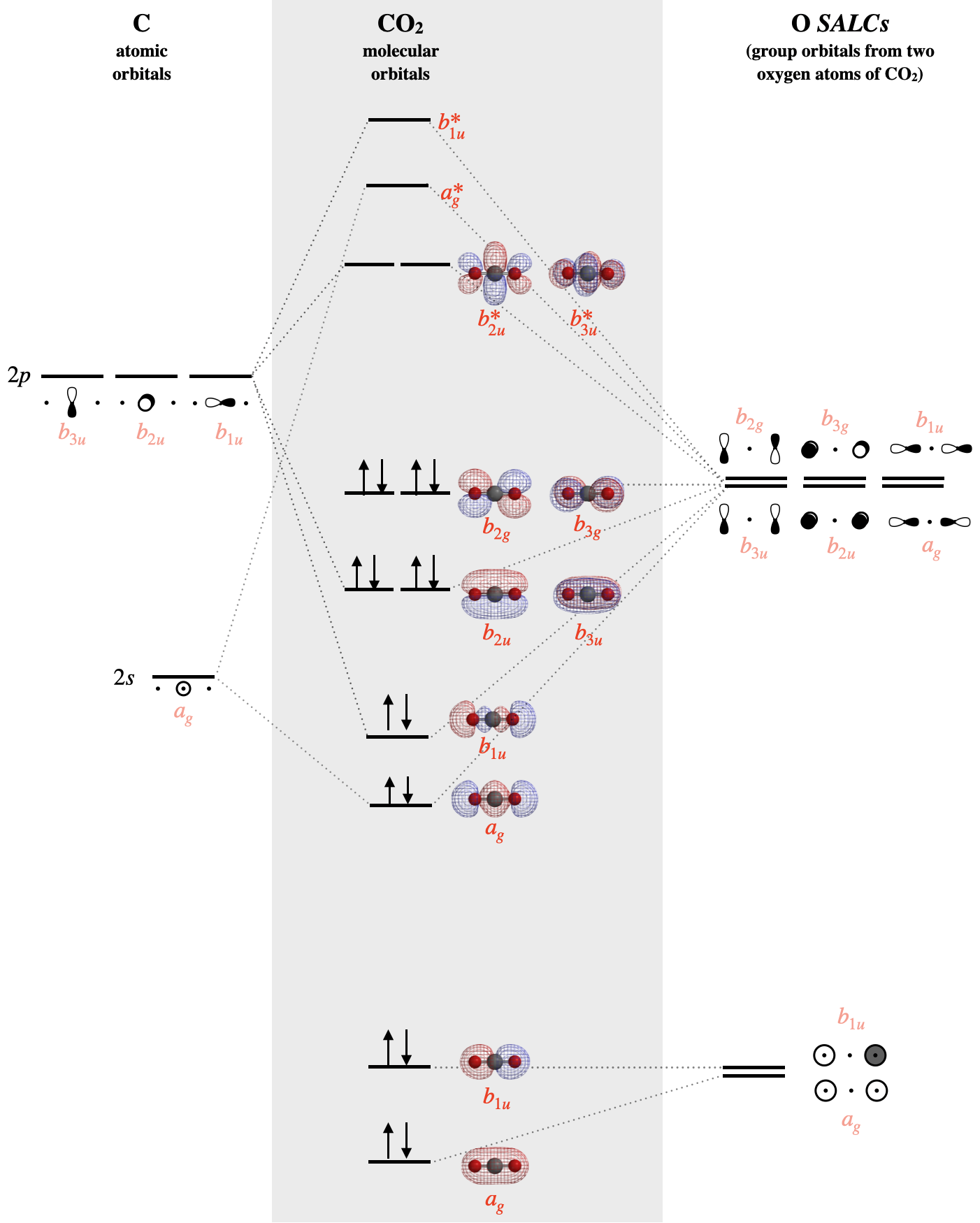
The SALCs on the right side of the diagram above are constructed from groups of either the \(2s\) atomic orbitals of oxygen, or the \(2p\) atomic orbitals of oxygen. Each SALC will combine with the atomic orbitals of carbon that have compatible symmetry; but the strength of the interaction depends on their relative energies. The individual valence atomic orbitals of oxygen have energies of \(-32.36 eV\) (\(2s\)) and \(-15.87 eV\) (\(2p\)), while the valence orbitals of carbon have energies of \(-19.47 eV\) (\(2s\)) and \(-10.66 eV\) (\(2p\)). The \(2s\) orbitals of the oxygen are far lower in energy (\(-32.36 eV\)) than all other valence orbitals, and so we should expect that molecular orbitals that are constructed from these oxygen \(2s\) will be mostly non-bonding. These mostly non-bonding orbitals are the \(a_{1g}\) and \(b_{1g}\) orbitals shown at the bottom of Figure \(\PageIndex{3}\). The \(a_g\) orbital is lower in energy than the \(b_{1u}\) due to slight mixing with other orbitals of \(a_g\) symmetry.

The bonding orbitals of \(CO_2\) include two \(sigma\) molecular orbitals of \(a_g\) and \(b_{1u}\) symmetry and two \(\pi\) molecular orbitals of \(b_{2u}\) and \(b_{3u}\) symmetry. Each of these bonding molecular orbitals possesses a higher-energy antibonding partner. The \(b_{2g}\) and \(b_{3g}\) SALCs that are formed from oxygen \(2p_x\) and \(2p_y\) orbitals have no compatible match with carbon valence orbitals; thus they form two \(b_{2g}\) and \(b_{3g}\) molecular orbitals, which are truly non-bonding and mostly oxygen in character. Still, notice that each orbital is spread across both oxygen atoms at once, and again we see that each non-bonding electron pair in the HOMO is very different in molecular orbital theory compared to Lewis theory. Each non-bonding pair is distributed over both oxygen atoms at once in molecular orbital theory, while in Lewis theory each lone pair is isolated to one atom or to localized bonds attached to that atom.