
4.6: Calculating Equilibrium Concentrations with the "x-is-small" Approximation
- Page ID
- 364665

- Identify systems where the x-is-small approximation can be used to solve equilibrium problems
- Manipulate initial concentrations to start at the "all reactant" or "all product" condition
Sometimes it is possible to use chemical insight to find solutions to equilibrium problems without actually solving a quadratic (or more complicated) equation. Most of these cases involve reactions for which the equilibrium constant is either very small (\(K ≤ 10^{−3}\)) or very large (\(K ≥ 10^3\)).
Recall that a small Kc means that very little of the reactants form products. This means that the change in the concentration in the system (defined as \(x\)) is essentially negligible compared with the initial concentration of a substance. Knowing this simplifies the calculations dramatically.
The "x-is-small" approximation is based on the idea that if the system can be arranged so it starts “close” to equilibrium, then if the change (x) is small compared to any initial concentrations, it can be neglected. Small is usually defined as resulting in an error of less than 5%.
\(\% \:change=\dfrac{x}{initial \:concentration}×100\%\)
Example \(\PageIndex{1}\) demonstrates how the x-is-small approximation is used to simplify an equilibrium problem.
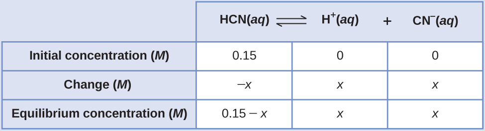
What are the concentrations at equilibrium of a 0.15 M solution of HCN?
Solution
Using “x” to represent the concentration of each product at equilibrium gives this ICE table.
The exact solution may be obtained using the quadratic formula with
solving
\[x^2+4.9×10^{−10}−7.35×10^{−11}=0\]
Thus [H+] = [CN–] = x = 8.6 × 10⁻⁶ M and [HCN] = 0.15 – x = 0.15 M.
In this case, chemical intuition can provide a simpler solution. From the equilibrium constant and the initial conditions, x must be small compared to 0.15 M. More formally, if \(x≪0.15\), then 0.15 – x ≈ 0.15. If this assumption is true, then it simplifies obtaining x
\[K_c=\dfrac{(x)(x)}{0.15−x}≈\dfrac{x^2}{0.15}\]
\[4.9×10^{−10}=\dfrac{x^2}{0.15}\]
\[x^2=(0.15)(4.9×10^{−10})=7.4×10^{−11}\]
\[x=\sqrt{7.4×10^{−11}}=8.6×10^{−6}\:M\]
In this example, solving the exact (quadratic) equation and using approximations gave the same result to two significant figures. While most of the time the approximation is a bit different from the exact solution, as long as the error is less than 5%, the approximate solution is considered valid. In this problem, the 5% applies to IF (0.15 – x) ≈ 0.15 M, so if
is less than 5%, as it is in this case, the assumption is valid. The approximate solution is thus a valid solution.
What are the equilibrium concentrations in a 0.25 M NH3 solution?
Assume that x is much less than 0.25 M and calculate the error in your assumption.
- Answer
-
\(\ce{[OH- ]}=\ce{[NH4+]}=0.0021\:M\); [NH3] = 0.25 M, error = 0.84%
Another type of problem that can be simplified by assuming that changes in concentration are negligible is one in which the equilibrium constant is very large (\(K \geq 10^3\)). A large equilibrium constant implies that the reactants are converted almost entirely to products, so we can assume that the reaction proceeds 100% to completion. When we solve this type of problem, we view the system as equilibrating from the products side of the reaction rather than the reactants side. If the initial concentrations of only the reactants are given, we use stoichiometry to predict the maximum amount of product that could be formed in the reaction. We use these adjusted concentrations as the "initial" conditions of the reaction in the ICE table. This approach is illustrated in Example \(\PageIndex{2}\).
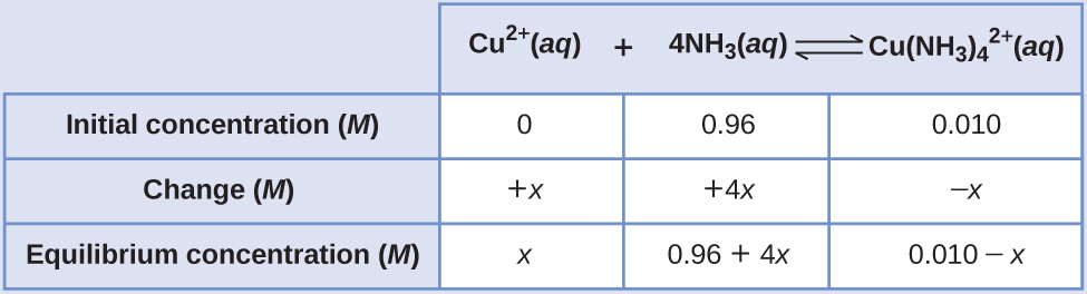
Copper(II) ions form a complex ion in the presence of ammonia
If 0.010 mol Cu2+ is added to 1.00 L of a solution that is 1.00 M NH3 what are the concentrations when the system comes to equilibrium?
Solution The initial concentration of copper(II) is 0.010 M. The equilibrium constant is very large so it would be better to start with as much product as possible because “all products” is much closer to equilibrium than “all reactants.” Note that Cu2+ is the limiting reactant; if all 0.010 M of it reacts to form product the concentrations would be
\[\ce{[Cu^2+]}=0.010−0.010=0\:M\]
\[\ce{[Cu(NH3)4^2+]}=0.010\:M\]
\[\ce{[NH3]}=1.00−4×0.010=0.96\:M\]
Using these “shifted” values as initial concentrations with x as the free copper(II) ion concentration at equilibrium gives this ICE table.
Since we are starting close to equilibrium, x should be small so that
Select the smallest concentration for the 5% rule.
This is much less than 5%, so the assumptions are valid. The concentrations at equilibrium are
By starting with the maximum amount of product, this system was near equilibrium and the change (x) was very small. With only a small change required to get to equilibrium, the equation for x was greatly simplified and gave a valid result well within the 5% error maximum.
What are the equilibrium concentrations when 0.25 mol Ni2+ is added to 1.00 L of 2.00 M NH3 solution?
\[\ce{Ni^2+}(aq)+\ce{6NH3}(aq)⇌\ce{Ni(NH3)6^2+}(aq) \nonumber \]
with \(K_c=5.5×10^8\).With such a large equilibrium constant, first form as much product as possible, then assume that only a small amount (x) of the product shifts left. Calculate the error in your assumption.
- Answer
-
\(\ce{[Ni(NH3)6^2+]}=0.25\:M\), [NH3] = 0.50 M, [Ni2+] = 2.9 × 10⁻⁸ M, error = 1.2 × 10⁻⁵%
Summary
When given the equilibrium constant and the initial concentrations, we can solve for the concentrations at equilibrium. When the equilibrium constant K is very small or very large, the mathematical operations can be simplified using the x-is-small approximation. When using the approximation, the x value from the equilibrium calculation should be less than 5% of any of the initial concentrations.