4.5: Calculating Equilibrium Constants and Equilibrium Concentrations

Learning Objectives

• To determine the equilibrium constant K from equilibrium concentrations.
• To calculate the equilibrium concentrations in a reaction when initial concentrations and K are know.

There are two fundamental kinds of equilibrium problems:

1. those in which we are given the concentrations of the reactants and the products at equilibrium (or, more often, information that allows us to calculate these concentrations), and we are asked to calculate the equilibrium constant for the reaction; and
2. those in which we are given the equilibrium constant and the initial concentrations of reactants, and we are asked to calculate the concentration of one or more substances at equilibrium. In this section, we describe methods for solving both kinds of problems.

Calculating an Equilibrium Constant from Equilibrium Concentrations

We'll begin by considering the the conversion of n-butane, an additive used to increase the volatility of gasoline, into isobutane (2-methylpropane).

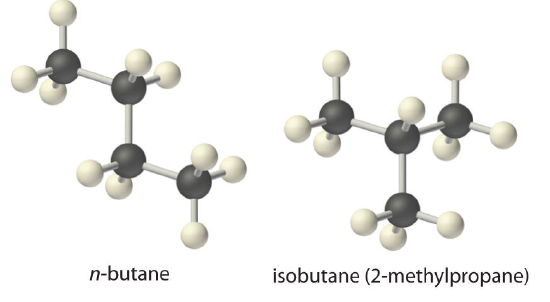
This reaction can be written as follows:

\[\ce{n-butane_{(g)} \rightleftharpoons isobutane_{(g)}} \label{Eq1}\]

and the equilibrium constant

\(K = [\text{isobutane}]/[\text{n-butane}]\).

At equilibrium, a mixture of n-butane and isobutane at room temperature was found to contain 0.041 M isobutane and 0.016 M n-butane. Substituting these concentrations into the equilibrium constant expression,

\[K=\dfrac{[\textit{isobutane}]}{[\textit{n-butane}]}=0.041\; M = 2.6 \label{Eq2}\]

Thus the equilibrium constant for the reaction as written is 2.6.

Example \(\PageIndex{1}\)

The reaction between gaseous sulfur dioxide and oxygen is a key step in the industrial synthesis of sulfuric acid:

\[2SO_{2(g)} + O_{2(g)} \rightleftharpoons 2SO_{3(g)}\nonumber\]

A mixture of \(SO_2\) and \(O_2\) was maintained at 800 K until the system reached equilibrium. The equilibrium mixture contained

• \(5.0 \times 10^{-2}\; M\; SO_3\),
• \(3.5 \times 10^{-3}\; M\; O_2\), and
• \(3.0 \times 10^{-3}\; M\; SO_2\).

Calculate \(K\) and \(K_p\) at this temperature.

Solution

Substituting the appropriate equilibrium concentrations into the equilibrium constant expression,

\[K=\dfrac{[SO_3]^2}{[SO_2]^2[O_2]}=\dfrac{(5.0 \times 10^{-2})^2}{(3.0 \times 10^{-3})^2(3.5 \times 10^{-3})}=7.9 \times 10^4 \nonumber\]

To solve for \(K_p\), we use the relationship derived previously

\[K_p = K(RT)^{Δn} \]

where \(Δn = 2 − 3 = −1\):

\[K_p=K(RT)^{Δn}\nonumber\]

\[K_p=7.9 \times 10^4 [(0.08206\; L⋅atm/mol⋅K)(800 K)]^{−1}\nonumber\]

\[K_p=1.2 \times 10^3\nonumber\]

Exercise \(\PageIndex{1}\)

Hydrogen gas and iodine react to form hydrogen iodide via the reaction

\[H_{2(g)}+I_{2(g)} \rightleftharpoons 2HI_{(g)}\nonumber\]

A mixture of \(H_2\) and \(I_2\) was maintained at 740 K until the system reached equilibrium. The equilibrium mixture contained

• \(1.37\times 10^{−2}\; M\; HI\),
• \(6.47 \times 10^{−3}\; M\; H_2\), and
• \(5.94 \times 10^{-4}\; M\; I_2\).

Calculate \(K\) and \(K_p\) for this reaction.

Answer

\(K = 48.8\) and \(K_p = 48.8\)

Since the law of mass action is the only equation we have to describe the relationship between K_c and the concentrations of reactants and products, any problem that requires us to solve for K_c must provide enough information to determine the reactant and product concentrations at equilibrium. Armed with the concentrations, we can solve the equation for K_c, as it will be the only unknown.

Example \(\PageIndex{1}\) showed us how to determine the equilibrium constant of a reaction if we know the concentrations of reactants and products at equilibrium. The following example shows how to use the stoichiometry of the reaction and a combination of initial concentrations and equilibrium concentrations to determine an equilibrium constant. This technique, commonly called an ICE table—for Initial, Change, and Equilibrium–will be helpful in solving many equilibrium problems. A chart is generated beginning with the equilibrium reaction in question. Underneath the reaction the initial concentrations of the reactants and products are listed—these conditions are usually provided in the problem and we consider no shift toward equilibrium to have happened. The next row of data is the change that occurs as the system shifts toward equilibrium. If the reaction shifts to the right, the change will be positive for the products (products are generated) and negative for the reactants (reactants are consumed). Importantly, we must consider the reaction stoichiometry when determining the quantities in the change row. If a reaction generates two moles of product for every mole of reactant, we must multiply the change quantity by two for the product side. The last row contains the concentrations once equilibrium has been reached, and will be the sum of the initial and change rows. Example \(\PageIndex{2}\) demonstrates how to use an ICE table to calculate the equilibrium constant.

Example \(\PageIndex{2}\)

A 1.00 mol sample of \(NOCl\) was placed in a 2.00 L reactor and heated to 227°C until the system reached equilibrium. The contents of the reactor were then analyzed and found to contain 0.056 mol of \(Cl_2\). Calculate \(K\) at this temperature. The equation for the decomposition of \(NOCl\) to \(NO\) and \(Cl_2\) is as follows:

\[2 NOCl_{(g)} \rightleftharpoons 2NO_{(g)}+Cl_{2(g)}\nonumber\]

Strategy:

1. Write the equilibrium constant expression for the reaction. Construct a table showing the initial concentrations, the changes in concentrations, and the final concentrations (as initial concentrations plus changes in concentrations).
2. Calculate all possible initial concentrations from the data given and insert them in the table.
3. Use the coefficients in the balanced chemical equation to obtain the changes in concentration of all other substances in the reaction. Insert those concentration changes in the table.
4. Obtain the final concentrations by summing the columns. Calculate the equilibrium constant for the reaction.

Solution

A The first step in any such problem is to balance the chemical equation for the reaction (if it is not already balanced) and use it to derive the equilibrium constant expression. In this case, the equation is already balanced, and the equilibrium constant expression is as follows:

\[K=\dfrac{[NO]^2[Cl_2]}{[NOCl]^2}\nonumber\]

To obtain the concentrations of \(NOCl\), \(NO\), and \(Cl_2\) at equilibrium, we construct a table showing what is known and what needs to be calculated. We begin by writing the balanced chemical equation at the top of the table, followed by three lines corresponding to the initial concentrations, the changes in concentrations required to get from the initial to the final state, and the final concentrations.

\[2 NOCl_{(g)} \rightleftharpoons 2NO_{(g)}+Cl_{2(g)}\nonumber\]

ICE	\([NOCl]\)	\([NO]\)	\([Cl_2]\)
Initial
Change
Final

B Initially, the system contains 1.00 mol of \(NOCl\) in a 2.00 L container. Thus \([NOCl]_i = 1.00\; mol/2.00\; L = 0.500\; M\). The initial concentrations of \(NO\) and \(Cl_2\) are \(0\; M\) because initially no products are present. Moreover, we are told that at equilibrium the system contains 0.056 mol of \(Cl_2\) in a 2.00 L container, so \([Cl_2]_f = 0.056 \;mol/2.00 \;L = 0.028\; M\). We insert these values into the following table:

\[2 NOCl_{(g)} \rightleftharpoons 2NO_{(g)}+Cl_{2(g)}\nonumber\]

ICE	\([NOCl]\)	\([NO]\)	\([Cl_2]\)
Initial	0.500	0	0
Change
Final			0.028

C We use the stoichiometric relationships given in the balanced chemical equation to find the change in the concentration of \(Cl_2\), the substance for which initial and final concentrations are known:

\[Δ[Cl_2] = 0.028 \;M_{(final)} − 0.00\; M_{(initial)}] = +0.028\; M\nonumber\]

According to the coefficients in the balanced chemical equation, 2 mol of \(NO\) are produced for every 1 mol of \(Cl_2\), so the change in the \(NO\) concentration is as follows:

\[Δ[NO]=\left(\dfrac{0.028\; \cancel{mol \;Cl_2}}{ L}\right)\left(\dfrac{2\; mol\; NO}{1 \cancel{\;mol \;Cl_2}}\right)=0.056\; M\nonumber\]

Similarly, 2 mol of \(NOCl\) are consumed for every 1 mol of \(Cl_2\) produced, so the change in the \(NOCl\) concentration is as follows:

\[Δ[NOCl]= \left(\dfrac{0.028\; \cancel{mol\; Cl_2}}{L}\right) \left(\dfrac{−2\; mol \;NOCl}{1\; \cancel{mol\; Cl_2}} \right) = -0.056 \;M\nonumber\]

We insert these values into our table:

\[2 NOCl_{(g)} \rightleftharpoons 2NO_{(g)}+Cl_{2(g)}\nonumber\]

ICE	\([NOCl]\)	\([NO]\)	\([Cl_2]\)
Initial	0.500	0	0
Change	−0.056	+0.056	+0.028
Final			0.028

D We sum the numbers in the \([NOCl]\) and \([NO]\) columns to obtain the final concentrations of \(NO\) and \(NOCl\):

\[[NO]_f = 0.000\; M + 0.056 \;M = 0.056\; M\nonumber\]

\[[NOCl]_f = 0.500\; M + (−0.056\; M) = 0.444 M\nonumber\]

We can now complete the table:

\[2 NOCl_{(g)} \rightleftharpoons 2NO_{(g)}+Cl_{2(g)}\nonumber\]

ICE	\([NOCl]	\([NO]\)	\([Cl_2]\)
initial	0.500	0	0
change	−0.056	+0.056	+0.028
final	0.444	0.056	0.028

We can now calculate the equilibrium constant for the reaction:

\[K=\dfrac{[NO]^2[Cl_2]}{[NOCl]^2}=\dfrac{(0.056)^2(0.028)}{(0.444)^2}=4.5 \times 10^{−4}\nonumber\]

Exercise \(\PageIndex{2}\)

The German chemist Fritz Haber (1868–1934; Nobel Prize in Chemistry 1918) was able to synthesize ammonia (\(NH_3\)) by reacting \(0.1248\; M \;H_2\) and \(0.0416\; M \;N_2\) at about 500°C. At equilibrium, the mixture contained 0.00272 M \(NH_3\). What is \(K\) for the reaction

\[N_2+3H_2 \rightleftharpoons 2NH_3\nonumber\]

at this temperature? What is \(K_p\)?

Answer

\(K = 0.105\) and \(K_p = 2.61 \times 10^{-5}\)

A Video Disucssing Using ICE Tables to find Kc: https://youtu.be/CwQmO4M2s64

Calculating Equilibrium Concentrations from the Equilibrium Constant

To describe how to calculate equilibrium concentrations from an equilibrium constant, we will again consider a system that contains only a single product and a single reactant, the conversion of n-butane to isobutane (Equation \(\ref{Eq1}\)), for which K = 2.6 at 25°C. If we begin with a 1.00 M sample of n-butane, we can determine the concentration of n-butane and isobutane at equilibrium by constructing an ICE table, just as we did in Example \(\PageIndex{2}\).

\[\text{n-butane}_{(g)} \rightleftharpoons \text{isobutane}_{(g)}\]

ICE	\([\text{n-butane}_{(g)} ]\)	\([\text{isobutane}_{(g)}]\)
Initial
Change
Final

The initial concentrations of the reactant and product are both known: [n-butane]i = 1.00 M and [isobutane]i = 0 M. We need to calculate the equilibrium concentrations of both n-butane and isobutane. Because it is generally difficult to calculate final concentrations directly, we focus on the change in the concentrations of the substances between the initial and the final (equilibrium) conditions. We know this reaction will generate products as it approaches equilibrium because initially no isobutane is present. If, for example, we define the change in the concentration of isobutane (Δ[isobutane]) as \(+x\), then the change in the concentration of n-butane is Δ[n-butane] = \(−x\). This is because the balanced chemical equation for the reaction tells us that 1 mol of n-butane is consumed for every 1 mol of isobutane produced. We can then express the final concentrations in terms of the initial concentrations and the changes they have undergone.

\[\text{n-butane}_{(g)} \rightleftharpoons \text{isobutane}_{(g)}\]

ICE	\([\text{n-butane}_{(g)} ]\)	\([\text{isobutane}_{(g)}]\)
Initial	1.00	0
Change	\(−x\)	\(+x\)
Final	\((1.00 − x)\)	\((0 + x) = x\)

Substituting the expressions for the final concentrations of n-butane and isobutane from the table into the equilibrium equation,

\[K=\dfrac{[\text{isobutane}]}{[\text{n-butane}]}=\dfrac{x}{1.00−x}=2.6\]

Rearranging and solving for \(x\),

\[x=2.6(1.00−x)= 2.6−2.6x\]

\[x+2.6x= 2.6\]

\[x=0.72\]

We obtain the final concentrations by substituting this \(x\) value into the expressions for the final concentrations of n-butane and isobutane listed in the table:

\[[\text{n-butane}]_f = (1.00 − x) M = (1.00 − 0.72) M = 0.28\; M\]

\[[\text{isobutane}]_f = (0.00 + x) M = (0.00 + 0.72) M = 0.72\; M\]

We can check the results by substituting them back into the equilibrium constant expression to see whether they give the same \(K\) that we used in the calculation:

\[K=\dfrac{[\text{isobutane}]}{[\text{n-butane}]}=\left(\dfrac{0.72\; \cancel{M}}{0.28\;\cancel{M}}\right) =2.6\]

This is the same \(K\) we were given, so we can be confident of our results.

Example \(\PageIndex{3}\) illustrates a common type of equilibrium problem that you are likely to encounter.

Example \(\PageIndex{3}\): The water–gas shift reaction

The water–gas shift reaction is important in several chemical processes, such as the production of H₂ for fuel cells. This reaction can be written as follows:

\[H_{2(g)}+CO_{2(g)} \rightleftharpoons H_2O_{(g)}+CO_{(g)}\nonumber\]

\(K = 0.106\) at 700 K. If a mixture of gases that initially contains 0.0150 M \(H_2\) and 0.0150 M \(CO_2\) is allowed to equilibrate at 700 K, what are the final concentrations of all substances present?

Strategy:

1. Construct a table showing what is known and what needs to be calculated. Define \(x\) as the change in the concentration of one substance. Then use the reaction stoichiometry to express the changes in the concentrations of the other substances in terms of \(x\). From the values in the table, calculate the final concentrations.
2. Write the equilibrium equation for the reaction. Substitute appropriate values from the ICE table to obtain \(x\).
3. Calculate the final concentrations of all species present. Check your answers by substituting these values into the equilibrium constant expression to obtain \(K\).

Solution

A The initial concentrations of the reactants are \([H_2]_i = [CO_2]_i = 0.0150\; M\). Just as before, we will focus on the change in the concentrations of the various substances between the initial and final states. If we define the change in the concentration of \(H_2O\) as \(x\), then \(Δ[H_2O] = +x\). We can use the stoichiometry of the reaction to express the changes in the concentrations of the other substances in terms of \(x\). For example, 1 mol of \(CO\) is produced for every 1 mol of \(H_2O\), so the change in the \(CO\) concentration can be expressed as \(Δ[CO] = +x\). Similarly, for every 1 mol of \(H_2O\) produced, 1 mol each of \(H_2\) and \(CO_2\) are consumed, so the change in the concentration of the reactants is \(Δ[H_2] = Δ[CO_2] = −x\). We enter the values in the following table and calculate the final concentrations.

\[H_{2(g)}+CO_{2(g)} \rightleftharpoons H_2O_{(g)}+CO_{(g)}\nonumber\]

ICE	\([H_2]\)	\([CO_2]\)	\([H_2O]\)	\([CO]\)
Initial	0.0150	0.0150	0	0
Change	\(−x\)	\(−x\)	\(+x\)	\(+x\)
Final	\((0.0150 − x)\)	\((0.0150 − x)\)	\(x\)	\(x\)

B We can now use the equilibrium equation and the given \(K\) to solve for \(x\):

\[K=\dfrac{[H_2O][CO]}{[H_2][CO_2]}=\dfrac{(x)(x)}{(0.0150−x)(0.0150−x}=\dfrac{x^2}{(0.0150−x)^2}=0.106\nonumber\]

We could solve this equation with the quadratic formula, but it is far easier to solve for \(x\) by recognizing that the left side of the equation is a perfect square; that is,

\[\dfrac{x^2}{(0.0150−x)^2}=\left(\dfrac{x}{0.0150−x}\right)^2=0.106\nonumber\]

Taking the square root of the middle and right terms,

\[\dfrac{x}{(0.0150−x)} =(0.106)^{1/2}=0.326\nonumber\]

\[x =(0.326)(0.0150)−0.326x\nonumber\]

\[1.326x=0.00489\nonumber\]

\[x =0.00369=3.69 \times 10^{−3}\nonumber\]

C The final concentrations of all species in the reaction mixture are as follows:

• \([H_2]_f=[H_2]_i+Δ[H_2]=(0.0150−0.00369) \;M=0.0113\; M\)
• \([CO_2]_f =[CO_2]_i+Δ[CO_2]=(0.0150−0.00369)\; M=0.0113\; M\)
• \([H_2O]_f=[H_2O]_i+Δ[H_2O]=(0+0.00369) \;M=0.00369\; M\)
• \([CO]_f=[CO]_i+Δ[CO]=(0+0.00369)\; M=0.00369 \;M\)

We can check our work by inserting the calculated values back into the equilibrium constant expression:

\[K=\dfrac{[H_2O][CO]}{[H_2][CO_2]}=\dfrac{(0.00369)^2}{(0.0113)^2}=0.107\nonumber\]

To two significant figures, this K is the same as the value given in the problem, so our answer is confirmed.

Exercise \(\PageIndex{3}\)

Hydrogen gas reacts with iodine vapor to give hydrogen iodide according to the following chemical equation:

\[H_{2(g)}+I_{2(g)} \rightleftharpoons 2HI_{(g)}\nonumber\]

\(K = 54\) at 425°C. If 0.172 M \(H_2\) and \(I_2\) are injected into a reactor and maintained at 425°C until the system equilibrates, what is the final concentration of each substance in the reaction mixture?

Answer

• \([HI]_f = 0.270 \;M\)
• \([H_2]_f = [I_2]_f = 0.037\; M\)

In Example \(\PageIndex{3}\), the initial concentrations of the reactants were the same, which gave us an equation that was a perfect square and simplified our calculations. Often, however, the initial concentrations of the reactants are not the same, and/or one or more of the products may be present when the reaction starts. Under these conditions, there is usually no way to simplify the problem, and we must determine the equilibrium concentrations with other means. One way we can solve for \(x\) in the \(K\) expression is using the quadratic formula. Such a case is described in Example \(\PageIndex{4}\).

Example \(\PageIndex{4}\)

In the water–gas shift reaction shown in Example \(\PageIndex{3}\), a sample containing 0.632 M CO2 and 0.570 M \(H_2\) is allowed to equilibrate at 700 K. At this temperature, \(K = 0.106\). What is the composition of the reaction mixture at equilibrium?

Strategy:

1. Write the equilibrium equation. Construct a table showing the initial concentrations of all substances in the mixture. Complete the table showing the changes in the concentrations (\(x) and the final concentrations.
2. Write the equilibrium constant expression for the reaction. Substitute the known K value and the final concentrations to solve for \(x\).
3. Calculate the final concentration of each substance in the reaction mixture. Check your answers by substituting these values into the equilibrium constant expression to obtain \(K\).

Solution

A \([CO_2]_i = 0.632\; M\) and \([H_2]_i = 0.570\; M\). Again, \(x\) is defined as the change in the concentration of \(H_2O\): \(Δ[H_2O] = +x\). Because 1 mol of \(CO\) is produced for every 1 mol of \(H_2O\), the change in the concentration of \(CO\) is the same as the change in the concentration of H2O, so Δ[CO] = +x. Similarly, because 1 mol each of \(H_2\) and \(CO_2\) are consumed for every 1 mol of \(H_2O\) produced, \(Δ[H_2] = Δ[CO_2] = −x\). The final concentrations are the sums of the initial concentrations and the changes in concentrations at equilibrium.

\[H_{2(g)}+CO_{2(g)} \rightleftharpoons H_2O_{(g)}+CO_{(g)}\nonumber\]

ICE	\(H_{2(g)}\)	\(CO_{2(g)}\)	\(H_2O_{(g)}\)	\(CO_{(g)}\)
Initial	0.570	0.632	0	0
Change	\(−x\)	\(−x\)	\(+x\)	\(+x\)
Final	\((0.570 − x)\)	\((0.632 − x)\)	\(x\)	\(x\)

B We can now use the equilibrium equation and the known \(K\) value to solve for \(x\):

\[K=\dfrac{[H_2O][CO]}{[H_2][CO_2]}=\dfrac{x^2}{(0.570−x)(0.632−x)}=0.106\nonumber\]

In contrast to Example \(\PageIndex{3}\), however, there is no obvious way to simplify this expression. Thus we must expand the expression and multiply both sides by the denominator:

\[x^2 = 0.106(0.360 − 1.202x + x^2)\nonumber\]

Collecting terms on one side of the equation,

\[0.894x^2 + 0.127x − 0.0382 = 0\nonumber\]

This equation can be solved using the quadratic formula:

\[ x = \dfrac{-b \pm \sqrt{b^2-4ac}}{2a} = \dfrac{−0.127 \pm \sqrt{(0.127)^2−4(0.894)(−0.0382)}}{2(0.894)}\nonumber\]

\[x =0.148 \text{ and } −0.290\nonumber\]

Only the answer with the positive value has any physical significance, so \(Δ[H_2O] = Δ[CO] = +0.148 M\), and \(Δ[H_2] = Δ[CO_2] = −0.148\; M\).

C The final concentrations of all species in the reaction mixture are as follows:

• \([H_2]_f[ = [H_2]_i+Δ[H_2]=0.570 \;M −0.148\; M=0.422 M\)
• \([CO_2]_f =[CO_2]_i+Δ[CO_2]=0.632 \;M−0.148 \;M=0.484 M\)
• \([H_2O]_f =[H_2O]_i+Δ[H_2O]=0\; M+0.148\; M =0.148\; M\)
• \([CO]_f=[CO]_i+Δ[CO]=0 M+0.148\;M=0.148 M\)

We can check our work by substituting these values into the equilibrium constant expression:

\[K=\dfrac{[H_2O][CO]}{[H_2][CO_2]}=\dfrac{(0.148)^2}{(0.422)(0.484)}=0.107\nonumber\]

Because \(K\) is essentially the same as the value given in the problem, our calculations are confirmed.

Exercise \(\PageIndex{4}\)

The reaction of hydrogen and iodine vapor to form hydrogen iodide, for which \(K = 54\) at 425°C, is shown below.

\[H_{2(g)}+I_{2(g)} \rightleftharpoons 2HI_{(g)}\nonumber\]

If a sample containing 0.200 M \(H_2\) and 0.0450 M \(I_2\) is allowed to equilibrate at 425°C, what is the final concentration of each substance in the reaction mixture?

Answer

• \([H_I]_f = 0.0882\; M\)
• \([H_2]_f = 0.156\; M\)
• \([I_2]_f = 9.2 \times 10^{−4} M\)

In many situations it is not necessary to solve a quadratic (or higher-order) equation. These types of equilibrium problems are described in the next section.

A Video Discussing Using ICE Tables to find Eq. Concentrations & Kc: https://youtu.be/vGQWZHlNWyM

Summary

Various methods can be used to solve the two fundamental types of equilibrium problems: (1) those in which we calculate the concentrations of reactants and products at equilibrium and (2) those in which we use the equilibrium constant and the initial concentrations of reactants to determine the composition of the equilibrium mixture. When an equilibrium constant is calculated from equilibrium concentrations, molar concentrations or partial pressures are substituted into the equilibrium constant expression for the reaction. Equilibrium constants can be used to calculate the equilibrium concentrations of reactants and products by using the quantities or concentrations of the reactants, the stoichiometry of the balanced chemical equation for the reaction, and a tabular format (i.e. an ICE table) to obtain the final concentrations of all species at equilibrium.