
1.2: The quantum-mechanical model of the atom
- Page ID
- 344568

Wave Particle Dualism
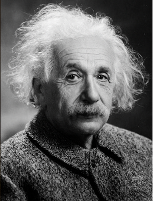
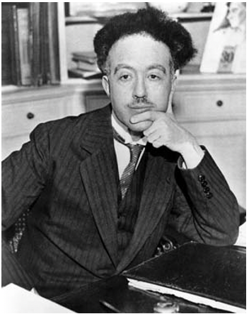
The phenomenon of the wave-particle dualism was first discovered for electromagnetic radiation, and the extended to all other particles including the electron. It began with the investigation of the photoelectric effect by Albert Einstein (Fig. 1.2.1 and Fig. 1.2.2).
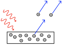
The photoelectric effect occur when a metal surface is irradiated by light. Above a certain frequency, or below a certain wavelength, light is able to eject electrons from the metal surface. The threshold frequency depends on the metal. Below the threshold frequency no electrons get ejected. Einstein investigated the maximum kinetic energy of the ejected electrons as a function of the frequency of the light. He found that there was a linear relationship. He analyzed the slope of this line and found that the slope was the Planck constant h. This would mean that electrons had an energy E=h\(\nu\) minus an energy EB that would be needed to overcome the binding energy, also called the work function, of the electron in the metal (Figure 1.2.3, left).
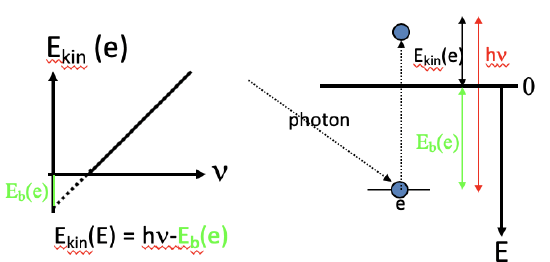
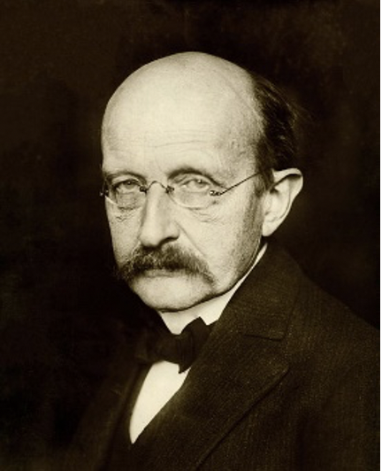
The equation E=h\(\nu\) was previously derived by Planck (Fig. 1.2.4) based on the assumption that energy was quantized, and now Einstein had experimentally found it again in the quest to explain the photoelectric effect. This would mean that light was quantized. The quantization would be explained by the fact that light would not only have wave but also particle properties, and these particles would be called photons. Assuming photons the photoelectric effect could be easily explained (Figure 1.2.3, right). When light hits the metal surface the photon collides with the electron. Only when the photon had an energy larger than the work function of the metal, the electron would be ejected and would have a kinetic energy equal to the difference between the energy of the photon and the binding energy. The wave-particle dualism of light, and electromagnetic radiation in general can also be mathematically derived. Because mass can be converted into electromagnetic radiation according to the equation E = mc2, and the energy of electromagnetic radiation is E=h\(\nu\), mc2=h\(\nu\). We can solve the equation for \(\nu\), and then it is \(\nu\)=mc2/h. With \(\nu\)=c/λ, and solved for λ, the equation becomes λ=h/mc. This equation shows the wave particle-dualism of electromagnetic radiation because it relates a wavelength to a mass. In fact, the mass of the particle associated with electromagnetic radiation, the photon, is inverse proportional to the wavelength of the electromagnetic radiation. The discovery of the wave-particle dualism of electromagnetic radiation was a radically new concept that is difficult to grasp intellectually up to this date because the human mind tends to see waves and particles to be mutually exclusive. However, it is one of the most fundamental principles of nature. As we will see later, not only electromagnetic radiation shows the wave particle dualism, but all particles including electrons.
Wave Particle Dualism of Massive Particles
The wave-particle dualism was originally thought to be valid for the photon only. A young French physics PhD student, Louis De Broglie had the radical idea that not only the photon, but all particles would exhibit the wave particle dualism, including the electron. Einstein’s formula λ = h/mc would just need to be slightly rearranged into λ = h/mv, whereby m would be the mass of the particle, and v would be the velocity of the particle. This idea was much disputed at the time, and Louis De Broglie’s PhD thesis was almost not accepted. However, eventually the wave-particle dualism of the electron was proven by electron diffraction experiments, and Louis De Broglie was awarded the Nobel prize in 1929. Today, we believe that all particles show the wave-particle dualism, and no experiment up to this date indicates an exception.
Standing Waves
With the discovery of the wave-particle dualism of the electron, and the observation of the quantization of electronic states in atoms led physicists focus on a field in physics in which waves are quantized. The field of standing waves (Fig. 1.2.6).
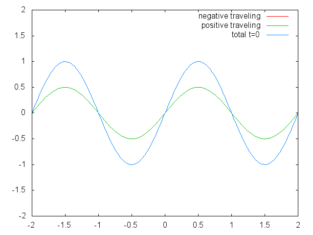
Figure 1.2.6 Two confined traveling waves (red and green) producing a standing wave (blue) due to their interference. (Attribution: Govindabalan [CC BY-SA (https://creativecommons.org/licenses/by-sa/3.0)], commons.wikimedia.org/wiki/F..._animation.gif)
Standing waves are a quite common phenomenon. You can for example trigger a standing waves by plucking a guitar string. This causes the guitar string to vibrate in standing waves with discreet, quantized wavelengths. The vibration with the longest wavelength is the so-called ground vibration. Its wavelength is two times the length of the guitar string. In addition, so-called higher harmonics are possible. The first harmonic has a wavelength equal to the length of the guitar string, the second one, has a wavelength equal to two-thirds of the length of the string, the third one has a wavelength equal to half of the length of the string, the fourth one has a wavelength equal to one third of the length of the guitar string, and so fourth (Fig. 1.2.7).

It can be easily seen that the possible wavelengths at which the string can vibrate follow the equation λ=2L/n, whereby n is an integer, or a quantum number, and L is the length of the guitar string. Thus, we can say that the waves associated with the guitar string vibrations are quantized. Why are these waves called standing waves? This is because the positions of the crests and the troughs and the nodes do not move. They remain at the same position on the guitar string at any point in time. It should be said here that the standing nature of the waves is actually an illusion. There are actually two waves traveling in opposite direction on the guitar string, and these waves interfere with each other so that a standing wave is produced (this is illustrated in Fig. 1.2.6). When the guitar string is plucked two waves are sent into opposite direction on the guitar string toward the two opposite ends on the guitar string. Once they have reached these ends they get reflected and sent into the opposite direction until they again reach the ends of the guitar string where they get reflected again. During this process, which happens over and over again, the two waves interfere and produce the standing wave. In sum, the fact that the wave is confined within the guitar string, leads to the quantized standing waves.
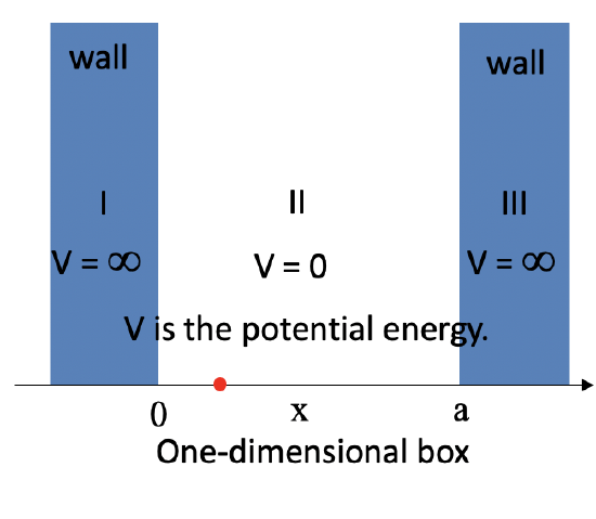
Electron in a One-Dimensional Box
Let us know go from a vibrating guitar string to an electron in a one-dimensional box of length a having infinitely high walls. Inside the box the potential energy of the electron is zero, in the walls the potential energy is infinite (Figure 1.2.8).
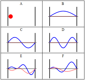
Due to its kinetic energy the electron can travel on a line within the box until it hits the wall (Fig. 1.2.9, A). At the wall it is getting reflected and forced to travel into the opposite direction until it again hits the wall where it reverses direction again, and so forth. Consider now that the electron does not only have particle, but also wave properties. Because of that also a wave travels along the line, gets reflected at the wall, travels into opposite direction, gets reflected again and so on. These waves can interfere with it other just like the waves traveling on the guitar string to produce a standing wave. Thus, the electron in the one-dimensional box should behave like a standing wave, and this wave should be quantized (Fig. 1.2.9, B-F).
How can we mathematically describe the electron in the box as a standing wave? Generally, you can describe a standing wave by a wave function. A wave function tells the amplitude of the standing wave at a particular position in the one-dimensional box. How can we find the wave function? We can start out from a differential equation that is generally valid for standing waves (Eq. 1.2.1).
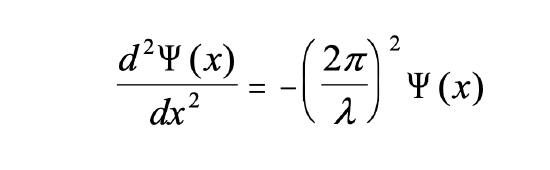
Equation 1.2.1 Standing wave differential equation.
It says that the second derivative of the amplitude of the wave function at the position x is equal to –(2π/λ)2 multiplied with the amplitude of the wave function at the position x. Let us now consider that the kinetic energy of the electron is E = 1/2mv2 and expand the equation by m.
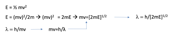
Equation 1.2.2 Solving for λ from kinetic energy equation and De Broglie equation.
Let us then solve the equation for (mv) . Now let us solve the De Broglie equation for mv and insert mv by h/λ in the previous equation. Finally, let us solve the equation by λ and we will get λ = h/[2mE]1/2, Eq. 1.2.2. We can now substitute λ by h/[2mE]1/2 in the differential equation. Slightly rearranged this equation becomes the Schrödinger equation for the electron in the one-dimensional box (Equation 1.2.3).
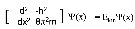
Equation 1.2.3 Schrödinger Equation for the electron in a 1-D box.
The Schrödinger equation is a differential equation. To get the wave function that describes the electron in the box we need to solve the differential equation. One possibility solve a differential equation is to guess its solution, and after that show that the solution is right. This is the approach we want to pursue here. A very general wave function is one that is a sum of a sinus term and a cosinus term of the coordinate x whereby we shall assume two general coefficients r and s in front of x, and two other general coefficients A and B in front of the sinus and the cosinus term, respectively.
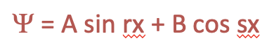
Equation 1.2.4 Generic solution to the differential equation.
We can now think of so-called boundary conditions for the wave function which will make the wave function more specific. A boundary condition is a property the wave function must have to be a sensible solution to the differential equation. We can assume a first boundary condition which assumes that at the position x=0 the amplitude of the wave function must be 0. This can be assumed because at these positions the "electron wave" gets reflected at the wall. That means that the wave function cannot have a cosinus term and thus B must be 0. If the wave function had a cosinus term it would not be 0 at x = 0 because the cosinus of 0 is not 0.

Equation 1.2.5 Boundary condition 1 for the wave function
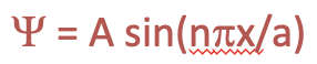
The second boundary condition is that the amplitude of the wave function is zero at x = a. Again, this is because the electron hits the wall at x = a and reverses its direction. The sinus function is only zero at x = a when ra is an integer number n times π: ra=nπ. This means that r must be nπ/a.

Equation 1.2.6 Boundary condition 2 for the wave function
Thus, the wave function must be A=sin(nπx/a). We can see that the wave function that describes the electron as a standing wave in the one-dimensional box is quantized because the quantum number n appears.
Equation 1.2.7 The wave function considering boundary conditions 1 and 2.
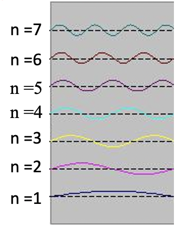
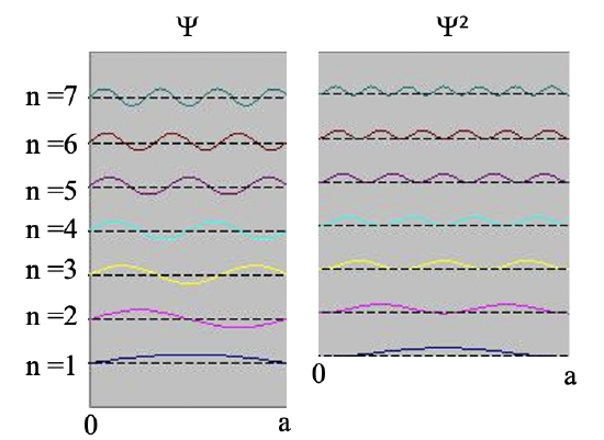
Inserting the quantum numbers n into the wave functions produces all the standing waves the electron can adopt (Fig. 1.2.10). You can see that the number of nodes and the wavelengths of the waves depend on the quantum number n. For n = 0 there is no node and the wavelength is twice the length of the box, for n = 2 there is one node and the wavelength is equal to the length of the box, for n =3 there are three nodes and the wavelength of the wave is 2/3 of the lengths of the box and so forth. We can illustrate that the wave function describes the waves depicted in Figure 1.2.10 by an example. The amplitude for the wave for n=2 is zero in the middle of the box where x = a/2. If we insert a/2 into the equation for Ψ then Ψ = A sin(nπ2a/a)= A sin(nπ) = 0 because it is the property of a sinus function to be 0 at an integer number multiple of π. We could also insert other values for x and n into the wave function, and would get the expected amplitude. This shows that the wave function correctly represents the standing waves the electron can adopt.
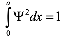
We are still not quite finished with the wave function because we have not determined the parameter A in front of the sinus term. To obtain it we need to consider a third boundary condition (Eq. 1.2.8).
Equation 1.2.8 Boundary condition 3.
It says that the integral of the square of the wave function over the length of the box must be equal to one. We can understand this boundary condition when we consider that the square of the wave function represents the probability to find the electron at a particular position in the box. The value the square of Ψ adopts at a position x within the box represents the probability to find the electron at this position when we consider the electron as a particle. This is called the Born interpretation of the wave function, named after the German physicist Max Born.
Because the probability to find the electron anywhere in the box must be 100%, the integral of the square of the wave function over the entire box must be 100% or 1. One can show, and we omit the necessary mathematical steps for clarity here, that the boundary condition is only fulfilled when A is equal to the square root of 2/a. The final wave function is then psi is equal to 2/a sin(nπx/a). The factor square root of 2/a is called the normalization constant of the wave function because it adjusts the amplitude of the wave function so that the probability to find the electron anywhere in the box is 100%.
The Schrödinger Equation for the H Atom
Let us now go from an electron in a 1-dimensional box to the electron in the hydrogen atom. What is similar and what is different between these two cases. A similarity is that the electron is confined in an atom just like the electron is confined in the 1D box. Thus, like in the 1-dimensional box the electron should behave like a standing wave. While in the one-dimensional box there is only one coordinate to consider, there are three coordinates to consider for the electron in the atom. This is because an atom is spherical and thus three coordinates x, y, and z are necessary to describe a position within the atom. A second major difference is that the potential energy of the electron is zero at any position within the box, while it is not zero in the hydrogen atom. This is because in an atom there are attractive Coulomb forces between the nucleus and the electron. The further away the electron is from the nucleus the higher its potential energy. This is because it takes energy to pull the electron away from the nucleus.
We therefore need to modify the Schrödinger equation that we used previously for the one-dimensional box the following way. Firstly, we need to expand the operator for the kinetic energy from one to three dimensions and introduce the coordinates y and z in addition to x. Secondly, we have to add an operator for the potential energy to the equation. The potential energy is the Coulomb energy between the proton and the electron. It is similar to the term we previously used for the calculation of the potential energy of the electron in the Bohr model. Instead of the radius r we use now the square root of the sum of the square of the three coordinates x, y, and z, to indicate the Coulomb energy of the electron at any position within the atom. Our wave function will now be a function of three coordinates x, y, and z. This means our wave function will now be three-dimensional and represent three-dimensional standing waves. Three-dimensional waves are harder to imagine compared to 1-dimensional ones, but have the same properties, which are that the position of the crests, troughs, and nodes does not move.
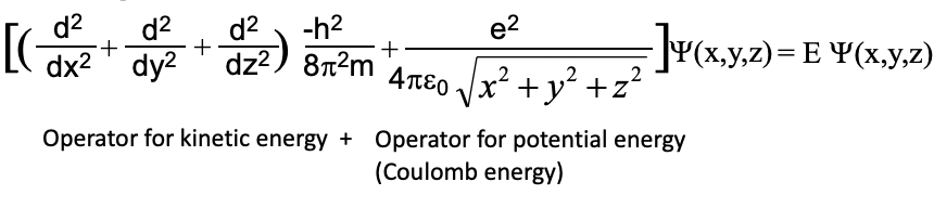
Equation 1.2.9 Schrödinger equation for the H atom.
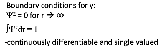
In order to get the wave functions for the electron we need to solve the Schrödinger equation for the hydrogen atom. To do so, we need to think about the boundary conditions for the wave function. One condition is that the square of the wave function approaches zero when we go very far from the nucleus, and r, the distance from the nucleus approaches infinite. Secondly, like in the one-dimensional box, the integral over the square of the wave function must be one. This is because the probability to find the electron somewhere in the atom must be 100%. Thirdly, it would be sensible to assume that the wave function must be continuously differentiable and single valued (Fig. 1.2.13).
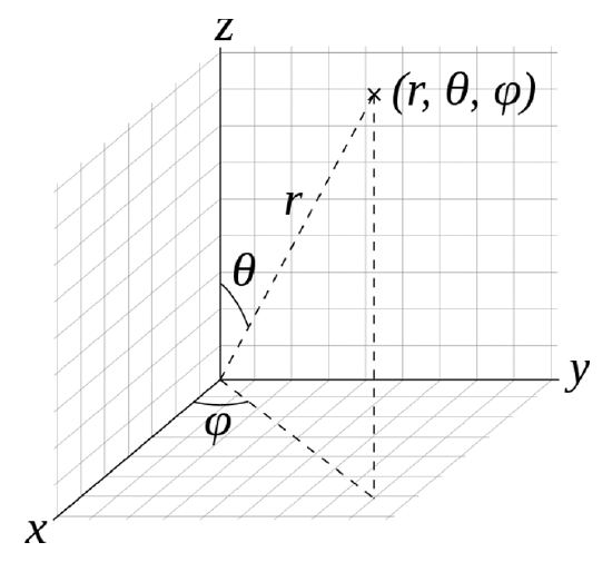
The Spherical Polar Coordinate System
The mathematical process to solve the Schrödinger equation is beyond the scope of this course and you are referred to Physical Chemistry classes and textbooks for the details. We shall only provide an brief outline of the process here. It is mathematically simpler to solve the Schrödinger equation in spherical polar coordinates instead of cartesian coordinates. Therefore, we obtain the solutions of the Schrödinger equation, the wavefunctions, in polar coordinates. The position of a point is specified by three numbers: the radial distance of that point from a fixed origin, its polar angle measured from a fixed zenith direction, and the azimuthal angle of its orthogonal projection on a reference plane that passes through the origin and is orthogonal to the zenith, measured from a fixed reference direction on that plane (Fig. 1.2.14).
Solutions of the Schrödinger Equation
The wavefunction is then a function of r, θ and φ, in particular it is a product of a radial wave function which is function of r, a colatitude wave function, which is a function of θ, and an azimuthal wave function which is a function of φ (Eq. 1.2.10). You can see the explicit forms of the radial, colatitude, and azimuthal functions in Fig. 1.2.15.
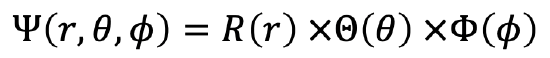
Equation 1.2.10 The wave function for the electron in the H atom as a function of r, θ and φ
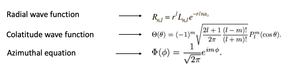
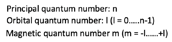
We do not need to understand all details here, but need to realize that these wavefunctions are functions of quantum numbers. In contrast to the electron in the one-dimensional box not only one, but three quantum numbers need to be considered. Beyond the quantum number n, which is the called the principal quantum number, there is also a so-called orbital quantum number l, and a magnetic quantum number m. The quantum number n only occurs in the radial wave function, the quantum number l only occurs in the radial and colatitude function, and the quantum number m only occurs in the colatitude and the azimuthal part of the wave function. The values the orbital quantum number l can adopt depends on n, it can be between 0 and n-1 for a given quantum number n. The magnetic quantum number m depends on the quantum number l, and can run from –l to +l. So, for example when n is equal to 2, l can vary between 0 and 1, and for l equal to 2, m can adopt any value between -2 and 2, namely -2,-1, 0, +1, and +2 (Fig. 1.2.16).
These wave functions have a particular name in chemistry. They are called orbitals. One can understand an orbital as the three-dimensional wave function that describes the electron in an atom as a standing wave. Thus, an orbital is a state the electron can adopt, and when we say that an electron is in a particular orbital we mean that the electron is in a particular state.
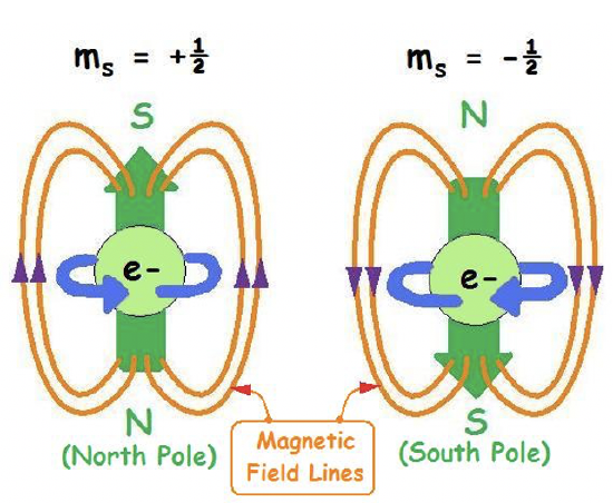
The spin quantum number s
Within an orbital an electron can adopt two different spins described by the spin quantum number s. This quantum number is not a result of the Schrödinger equation, but was found experimentally. The spin quantum number s can adopt two values: +1/2 and -1/2. We say an electron is spin up when s = +1/2, and spin down when s = -1/2.
chem.libretexts.org/@api/dek...jpg?revision=1, CC BY-NC-SA 3.0)
The spin quantum number is understood most easily when you view the electron as a particle rotating around its own axis. A counter-clockwise rotation would be associated with s=+1/2, a clockwise rotation would be associated with s=-1/2. The rotation produces a magnetic field with the direction of the field lines depending on the direction of rotation.
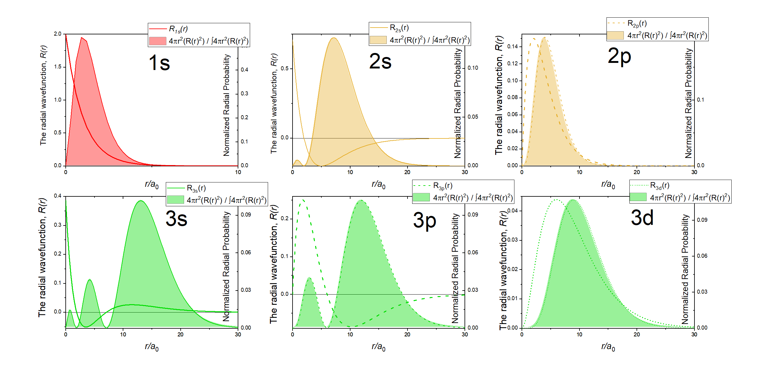
The 1s Orbital
Let us now insert the quantum numbers into the general form of the wave function for the electron in the hydrogen atom, and calculate their explicit mathematical forms. Let us start with the smallest possible numbers. When we insert n=1, l=0, and m=0 we get the wave function for the 1s orbital (Eq. 1.2.11).
Equation 1.2.11 Wave function for the 1s orbital
You can see that the colatitude and azimuthal parts of the wave functions, together also called the angular part of the wave function, are simple numbers, namely one over the square root of two pi, and one over the square root of two respectively. The angles theta and phi do not appear and that means that the wave function is angle-independent. This implies that the orbital has a spherical shape.
The radial part of the wave function has an exponential term e to the power of –r over a0. The number e is the Euler number, that is the base of the natural logarithm. It is approximately equal to 2.71828. a0 is the Bohr radius, which is the distance of the electron from the proton for the electron on its first orbit according to the Bohr atom model. We calculated it previously, and it was 5.29 x 10⁻¹¹m. r is the distance from the nucleus. This exponential term has a constant in front of it which is 1 over the Bohr radius to the power of three over two. Because the radial part of the wave function is e to the power of –r, the amplitude of the radial part of the wave function declines exponentially with increasing distance r from the nucleus. This is true for the entire wave function because the angular parts of the wave function are just simple numbers. You can see the exponential decline of the amplitude of the wave function as a function of the radius r in units of the Bohr radius a0 in the graph below (Fig. 1.2.19).
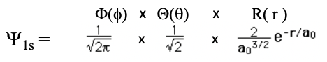
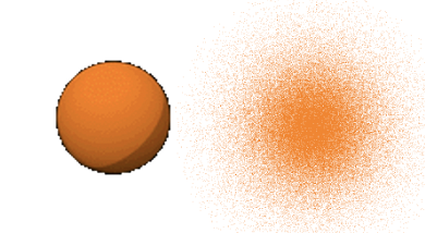
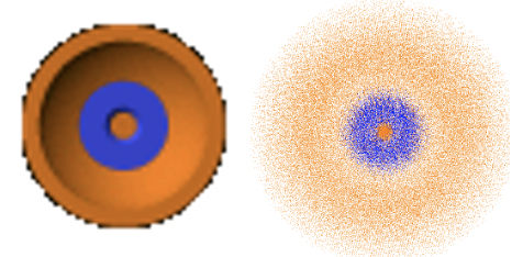
This means that the 1s orbital must be a spherical orbital with its amplitude exponentially declining with increasing distance from the nucleus. This can be graphically depicted via a density of points around the nucleus (Fig. 1.2.18). A higher density of points means higher amplitude and a lower density of points means smaller amplitude. The fact that the amplitude is the highest closest to the nucleus means that the probability to find the electron in a particular point in space is the highest closest to the nucleus. This is because the square of the wave function for the 1s orbital represents the probability to find the electron at a particular point in space. However, the probability to find the electron at a certain distance from the nucleus is not the highest closest to the nucleus. This is because the probability to find the electron at a certain distance from the nucleus is the probability to find the electron at a particular point in space times the number of points in space that have that particular distance. The number of points in space that have a particular distance r from the nucleus is related to the surface of a sphere with the a radius r. The surface of a sphere A is given by the formula A=4πr2. Thus, the probability to find the electron at a particular distance r from the nucleus is equal to the surface of a sphere with the radius r times the radial wave function square. This defines the radial probability function RP=4πr2R2.
The graph for the radial probability function is depicted in Figure 1.2.19. You can see that it is zero when r=0 which is due to the r2 term which becomes zero at r = 0. At small r values the 4πr2 term dominates the overall function and the probability to find the electron increases with r. However, because the exponential term of the radial function becomes more and more significant at larger r values, the radial probability function goes through a maximum and then declines. At distances r approaching infinite the function approaches zero. The maximum of the curve represents the distance at which it is most likely to find the electron. Interestingly, it is equal to the Bohr radius r. That means that Bohr was not so wrong after all. However, he was wrong in the sense that he viewed the electron as a classical particle being only at that radius. Instead, the electron, due to its wave properties, it is not only at the Bohr radius r0, but most likely we can find it there.
The result that the probability to find the electron at a specific point in space is the greatest at the nucleus does away with the question of why the H atom does not collapse. Because the amplitude of the wave function is the greatest closest to the nucleus we can actually say in a way that the atom is collapsed. Nonetheless, the atom is mostly empty space because of the delocalization of the wave function that describes the state of the electron. The delocalization of the electron due to its wave properties also makes the question of the size of an orbital non-trivial. The wave function approaches zero only for r approaching infinite, but never becomes zero. This means that to account for all electron density the orbital would be infinitely large. This however would not be a sensible definition. The commonly accepted definition is that the size of an orbital is defined by the space that contains 90% of its electron density. We can depict orbitals according to this definition. For the case of the 1s orbital the radius of the sphere that represents the 1s orbital is chosen so that the probability to find the electron within a sphere of that radius is 90%.
The 2s Orbital
Inserting n=2, l=0, and m=0 into the general wave function gives us the wave function for the 2s orbital (Eq. 1.2.12).
Equation 1.2.12 Wave function for the 2s orbital
Like in the case of the 1s orbital, the angular parts of the wave function are only simple numbers. Thus, the 2s orbital is also a spherical orbital. Like in the 1s orbital, the radial part of the wave function has an exponential term of the type e-r and a simple coefficient. However, there is an additional term 2-r/a0. Due to the exponential term, the amplitude of the wave function declines exponentially with r. However, because of the term 2-r/a0 the wave function becomes negative, and then approaches 0. The radius at which the wave function changes its algebraic sign is called a spherical node. The node is spherical because it describes the surface is a sphere. On the surface of this sphere the amplitude of the wave function is zero. The radius at which the wave function changes its algebraic sign is 2a0. This becomes clear when we consider that the term 2-r/a0 becomes zero when r=2a0 because 2-2a0/a0=0. When this term is zero then the entire wave function becomes zero. We can illustrate the change of the algebraic sign in the 2s orbital using colors as shown below (Fig. 1.2.20).

The orange sphere indicates the space in which the amplitude of the 2s orbital is positive, and the blue area indicates where it is negative. The interface area where the color changes represents the node. By multiplying the square of the radial wave function R with 4πr2 we obtain the radial probability function for the 2s orbital (Fig. 1.2.21).
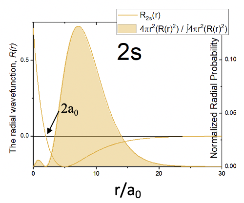
You can see that similar to the 1s orbital, the probability to find the electron on a radius closest to the nucleus is 0. However, unlike the 1s orbital there are now two maxima instead of only one. This second maximum is imposed by the spherical node of the 2s orbital. The second maximum is larger than the first one. Generally, the probability to find the electron further away from the nucleus is greater compared to the 1s orbital. That means that the 2s orbital is larger than the 1s orbital. This reflects the general trend that orbitals with a higher quantum number n tend to be larger and the probability to find the electron further away from the nucleus is greater.
The 3s Orbital
Let us look at one more s orbital, the 3s orbital (Eq. 1.2.13).
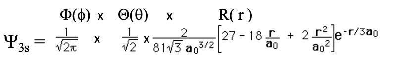
Equation 1.2.13 Wave function for the 3s orbital.
The angular parts of the wave function for the 3s orbital are again simple numbers, which implies that the orbital is again spherical. Generally all s orbitals are spherical.
The radial part of the wave function can be divided into the parts. The first part is a simple number, then there is the term 27-18r/a0+ 2r2/a02, and the exponential term e-r/3a0. Because of the exponential part the amplitude of the wave function declines exponentially with increasing r. However, then the wave function becomes negative, goes through a minimum, then becomes positive again, goes through a small maximum, and finally approaches zero. The fact that the wave function changes its algebraic sign two times means that the 3s orbital has two spherical nodes. These spherical nodes are due to the second term which is a square function of the type ax2 + bx + c, whereby in this case a = 2/a02, b =-18/a0 and c=27. When this term becomes zero the entire wave function becomes zero. Square functions have two solutions according the formula x=(-b±√(b2-4ac))/2a. The solutions give the radii for the two spherical nodes of the 3s orbital. We omit the exact calculation of the radii for briefness and clarity reasons here. You may calculate them as a homework.
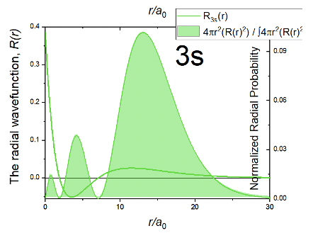
Because of the two spherical nodes, the radial probability function Rp has three maxima. A very small one close to the nucleus, are larger one further away from the nucleus, and the largest one at even greater distance from the nucleus. Overall, the 3s orbital is larger than the 2s orbital confirming the general trend that s orbitals increase in size with increasing quantum number n.
The 2pz Orbital
Now let us look at orbitals in which the orbital quantum number l is larger than 0. When l is equal to 1, then n must be at least 2. An orbital with n=2 and l=1 is a 2p orbital. Overall, three 2p orbitals must exist because for l=1, the magnetic quantum number m can adopt three values: -1, 0, and +1. The orbital with m=0 is called the 2pz orbital. Let us look at the mathematical form of this wave function (Eq. 1.2.14).
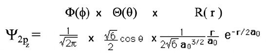
Equation 1.2.14 Wave function for the 2pz orbital
Analyzing the angular parts of the wave function shows that while the azimuthal part is still a simple number, the colatitude part is not, it is a function of θ. This means that the amplitude of the wave function is now angle dependent, which implies that the orbital cannot be spherical. Instead the 2p orbital has the shape of a dumbbell which is oriented along the z-axis. One lobe is above the xy plane, and the other lobe is below the xy plane. These two different lobes have a different algebraic sign, indicated by different colors (Fig. 1.2.24).
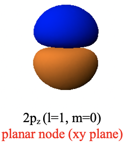
Within the xy plane the amplitude of the wave function is zero. The xy plane represents a so-called planar node. A planar node is a type of an angular node. The name angular node is because it is due to the fact that the angular part of the wave function is not a simple number, but a function of an angle, in this case θ. We can show that the angular part of the wave function produces the planar node in the xy plane when we convert it from spherical into Cartesian coordinates (Eq. 1.2.15).
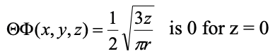
Equation 1.2.15 Angular part of the wave function of 2pz in cartesian coordinates. The function becomes zero when z=0.
We can see that the angular part of the wave function is only a function of z. We can also see, that the angular part of the wave function becomes zero when z=0. When the angular part of the wave function becomes zero, then the wave function of the entire orbital becomes zero. Z is zero only in the xy plane, and this explains why the xy plane is a planar node.
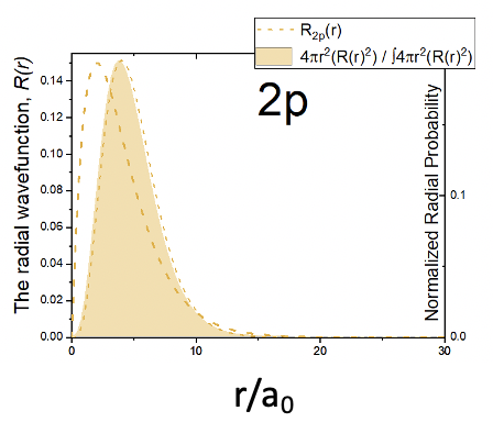
Now let us look at the radial part of the wave function. It is made of three terms: a simple constant, the term r/a0, and the exponential term e-r/2a0. Because of the term r/a0 the radial part of the wave function is zero at r=0. This means that it is very unlikely to find the electron at a point in space directly at the nucleus. This behavior is opposite to s orbitals. Because the r/a0 term dominates the behavior of the wave function at small r value, the amplitude first increases. However, at larger r values the exponential term becomes more an more important which forces the amplitude of the radial function through a maximum, after which it declines and approaches zero. The radial wave function never changes algebraic sign. Therefore, the 2pz orbital does not have a spherical node. The radial probability function has a similar shape compared to the radial function. It is zero at r=0 and goes through a maximum before it declines again and approaches zero (Figure 1.2.25).
The 2px and 2py Orbital
The 2px and the 2py orbitals are obtained when the quantum numbers m are 1, and -1, respectively.
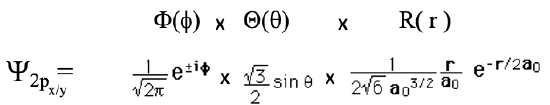
Equation 1.2.16 Wave function for the 2px and 2py orbital
They have the same shape as the 2pz orbital, but their orientation is different. The dumbbell of the 2px orbital is oriented along the x-axis, and that of the 2py orbital is oriented along the y-axis.
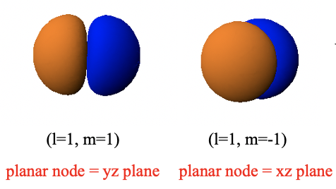
This is because the 2px orbital has a planar node in the yz plane, and the 2py orbital has a planar node in the xz plane. The planar nodes are due to the angular part of the wave functions of these orbitals.
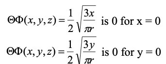
Equation 1.2.17 Angular part of the wave function of 2px and 2py, respectively. The wave functions become 0 for x=0 and y=0, respectively.
As one can see, the angular parts of the wave function contain both the angles θ and Φ. When converted into Cartesian coordinates (Eq. 1.2.17) one can see that the angular function of the 2px orbital is only a function of x, and the angular function of the 2py orbital is only a function of y. The functions become zero for x=0 and y=0, respectively. X is zero only in the yz plane, and y is zero only in the xz plane, hence these nodes are planar nodes. The radial wave function is exactly the same as for the 2pz orbital.
The 3p Orbitals
Now let us look at the 3p orbitals. In a 3p orbital the quantum number n=2 and l=1. Like for the case of the 2p orbitals there are three p orbitals because the magnetic quantum number m can adopt the values -1, 0, and +1. The wave function of the 3pz orbital is shown below (Eq. 1.2.18).
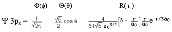
Equation 1.2.18 Wave function for the 3pz orbital
One can see that the angular part of the wave function is exactly the same as for the 2pz orbital. This means that like in the 2pz orbital there must be a planar node in the xy plane. When you look at the radial part of the wave function you can see that it is composed of four terms, a simple constant, a term 6-r/a0, the term r/a0, and the exponential term e-r/3a0. Because of the term r/a0 the wave function becomes zero at r=0. Because of the term 6-r/a0 the wave function has a spherical node. This is because when 6-r/a0=0 the entire wave function becomes 0. We can determine the radius at which the wave function becomes zero by solving the equation 6-r/a0=0 for r, which gives r=6a0. Overall, the radial function is zero at r=0, goes through a maximum, changes its algebraic sign at the spherical node at r=6a0, has a minimum, and then approaches zero for very large distances r (Fig. 1.2.28).
The radial probability function has two maxima, a small one close to the nucleus, and a larger one further away from the nucleus. Overall the radial probability function is further away from the nucleus compared to the 2p orbitals, which implies that the 3p orbital is larger.

The overall shape of the 3pz orbital is determined by the both the spherical and the planar node (Fig.1.2.29). Due to the planar node in the xy plane it has a dumbbell shape and is oriented in z direction. However, because of the spherical node the algebraic sign of the wave function changes within the two lobes of the dumbbell. Finally let us consider the 3px and the 3py orbitals. They would have the same shape as the 3pz orbital, but they would be oriented in the x and the y direction respectively. We could also think about what would happen to the p orbitals if we increased the quantum number n further. In this case the dumbbell shape would remain, but additional spherical nodes would be introduced. A 4p orbital would have two spherical nodes, a 5p orbital three spherical nodes, and so on. The size of these p orbitals would also increase with the quantum number n.
The 3dz2 Orbital
Now let us consider the orbitals with the orbital quantum number l=2. These orbitals are so-called d-orbitals. Because the principal quantum number n always has to be at least one integer number larger than the quantum l, the d orbitals with the smallest quantum number n are the 3d orbitals. For each quantum number n there must be five d orbitals because for l=2 the magnetic quantum number m can adopt the values -2, -1, 0, -1, +1, and +2. Let us first look at the 3d orbital with m=0. This orbital is called the 3dz2 orbital. Its wave function is shown below (Eq. 1.2.19).
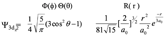
Equation 1.2.19 Wave function for the 3dz2 orbital
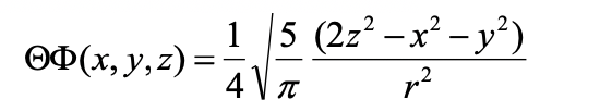
You can see that the radial function is a product of three terms: a constant, a term r2/a02, and the exponential term e-r/3a0. The exponential term is the same as for the 3p orbitals. Because of the term r2/a02 the amplitude of the wave function is 0 at r=0. The amplitude then increases with r, goes through a maximum, and then approaches zero. This means that the wave function never changes its algebraic sign, and therefore it does not have spherical nodes. The radial probability function has a similar shape compared to the radial function (Figure 1.2.30). The electron probability is somewhat further away from the nucleus compared to the 3p orbitals, meaning that the 3d orbital is somewhat larger than the 3p orbital.
You can see that the angular part of the wave function is a function of θ which means that the orbital will be non-spherical and there will be at least one angular node. In this case the angular nodes are two conical nodes. These nodes describe two cones that give the orbital its characteristic shape. It is a doughnut ring in the xy plane around a dumbbell pointing into z direction. The dumbbell and the doughnut have different algebraic signs indicated by different colors (Figure 1.2.31). Note that in contrast to the p orbitals the two lobes of the dumbbell have the same algebraic sign.
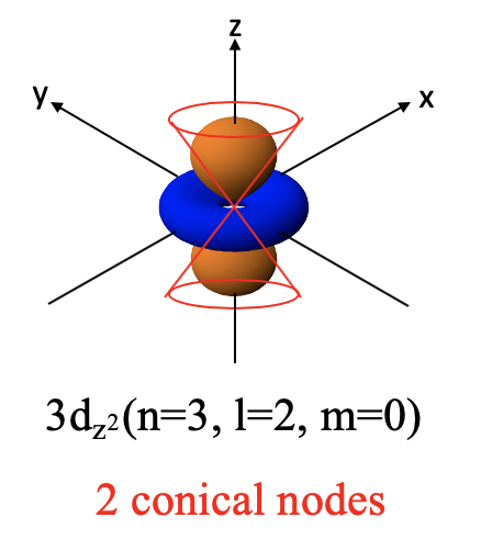
We can understand that the 3dz2 orbital has two conical nodes when we convert the angular part of the wave function into Cartesian coordinates (Eq. 1.2.20).
Equation 1.2.20 Angular part of the wave function of the 3dz2 orbital in cartesian coordinates.
You can see that it is a function of 2z2-x2-y2. This is the mathematical form of cones. The angular part of the wave function becomes 0 when 2z2=x2-y2 which is true on the surface of two cones, one above the xy plane and one below the xy plane. The name of the 3dz2 orbital is because it is a function of z2.
The 3dx2-y2 Orbital
Let us next look at the 3dx2-y2 orbital (Eq. 1.2.21).
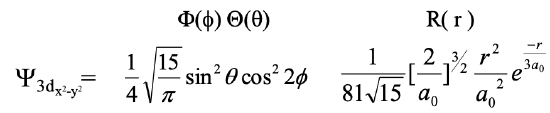
Equation 1.2.21 Wave function for the 3dx2-y2 orbital
The radial part of the wave function is the same as the one for the 3dz2 orbital. The angular part of the wave function is both a function of θ and Φ and thus there are angular nodes to expect. We can find them again when we convert the angular part of the wave function from spherical to Cartesian coordinates.
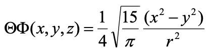
Equation 1.2.22 Angular part of the wave function of the 3dx2-y2 orbital in cartesian coordinates.
You can see that the angular function is a function of x2-y2. The function becomes zero when x2-y2=0. This is the case when x=y or x=-y. X is equal to y on two lines that bisect the 90 degree angle between the x and the y axis. The coordinate z is completely variable. Thus, overall, the wave function becomes zero on two planes that stand perpendicular to the xy plane and bisect the 90 degree angle between the x and the y axis. These two planes are therefore the two planar nodes of the orbital.
Because of the two planar nodes the orbital has four lobes lying on the x and the y axis, respectively. Lobes lying on the x-axis have the opposite algebraic sign compared to those lying on the y-axis. The name of the dx2-y2 orbital is because it is a function of x2-y2.
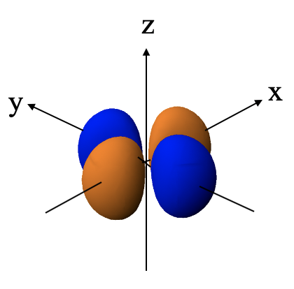
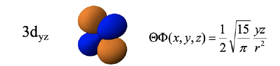
The 3dxy, 3dyz and 3dxz orbitals
The remaining d orbitals are the 3dyz, the 3dxz, and the 3dxy. The radial function of these orbitals is just like the ones we previously discussed. The angular part of the wave functions is shown here directly in Cartesian coordinates. The dyz orbital is a function of yz. The function becomes zero when either y=0 or z=0. y is zero in the xz plane, and z is zero in the xy plane. Therefore these planes are planar nodes of the orbital. Because of these nodes, the orbital has four lobes which lie in the yz plane whereby the lobes are in between the y and the z axes. Note that adjacent lobes have opposite algebraic sign, and opposite lobes have the same algebraic sign.
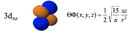
The 3dxz orbital is a function of xz, and thus the function becomes zero with x=0 or z=0. This defines that yz and the xy planes as the two planar nodes. The orbital has the same shape as the 3dyz, except that the four lobes lie within the xz plane instead the yz plane.
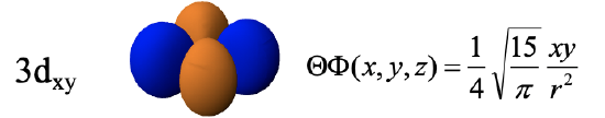
The 3dxy-orbital is a function of xy, and thus its wave function becomes zero at x=0 or y=0. Therefore, the xz and the yz planes are the planar nodes and the orbital has four lobes in the xy plane in between the x and the y axis. Note that the 3dxy and the 3dx2-y2 look very similar but are different. The difference is that the 3dx2-y2 orbital has its lobes on the x and the y axis, while the 3dxy orbital has the lobes in between the x and the y axis. One can also say that the 3dx2-y2 orbital is rotated by 45 degree around z with respect to the 3dxy orbital.
Rules for Angular and Spherical Nodes
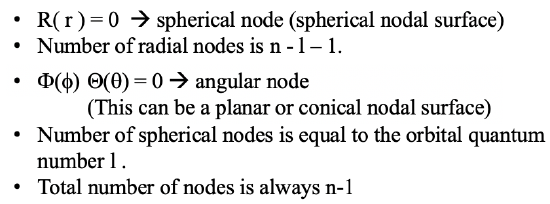
Of course, we could now discuss the size and shape of many other orbitals such a the 4d orbitals or the 4f orbitals, but this will be beyond scope. Instead, let us think about if there are general rules that allow the prediction of the number of spherical and angular nodes in an orbital. The number of radial nodes is always equal to n-l-1, the number of angular nodes is equal to l, and the total number of nodes is always n-1. This means that the number of nodes increases with the quantum number n. If we increase the quantum number l for a given quantum number n, then we replace spherical nodes by angular nodes. This is summarized in Figure 1.2.36.
The Orbital Energies for the H Atom
The Schrödinger equation does not only allow to calculate the orbitals of the hydrogen atom, but also their energies. The energies of Bohr and Schrödinger model match: E = constant/n2 : This means that orbitals with the same quantum number n have the same energies. The energies are not a function of the quantum numbers l and m. The energies are negative because they are binding energies. In other words: Adding an electron to a proton is an exothermic process. The binding energy for the energy increases as the orbital energy decreases (Fig. 1.2.37).

For the 1s orbital of H the energy is -13.6 eV, the energy of the 2s and the 2p orbitals are ¼ of that, the energy of the 3s, 3p, and 3d orbitals are 1/9 of the energy of the 1s orbital and so forth. Note at ¼ and 1/9th of -13.6 eV is more than -13.6 eV due to the negative algebraic sign. The electron volt is a unit of energy. It is the amount of kinetic energy gained by a single unbound electron when it passes through an electrostatic potential difference of one volt, in vacuum.

Equation 1.2.23 The electron volt to joule unit conversion.
In other words, it is equal to one volt (1 volt = 1 joule per coulomb) times the charge of a single electron (in coulombs). It is a very small unit of energy which is practical for orbital energy calculations because the orbital energies are very small (Eq. 1.2.23).
Multi-electron Atoms
Thus far we have only considered the orbitals for the hydrogen atom which contains only one electron. Can we also solve the Schrödinger equation for atoms that have more than one electron and get the exact energies of the orbitals? The answer is no, this mathematically not possible. The process is just already too complex even for only two electrons. The Schrödinger equation can only be solved for one electron systems. Therefore, the description of the atomic structure of all other atoms must work with approximations. Let us first consider the He atom. It has only one more electron than hydrogen. It is a useful approach to approximate multi-electron atoms as one-electron systems first, and then approximate the electron-electron interactions. Electron energies in an atom with more than one proton should follow the equation En=-Z2x13.6 eV/n2, whereby Z is the number of protons.
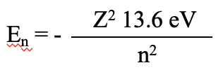
Equation 1.2.24 The orbital energies for atoms with more than one proton
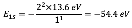
The binding energy of the electron increases proportionally to the square of the number of protons because the attractive Coulomb forces that act on the negatively charged electrons increases with the number of positively charged protons in the nucleus. One can experimentally measure the orbital energies via ionization energies. The energy required to remove an electron in a particular orbital from the atom is equal to the binding energy for the electron in that orbital. Therefore the ionization energy IE = -En (En = orbital energy). According to the Schrödinger model the orbital energy for a helium electron in a 1s orbital should be E1s=-(22×13.6 eV)/11 =-54.4 eV (Eq. 1.2.25).
Equation 1.2.25 Energy for a helium electron in a 1s orbital.
However, the experimentally measured ionization energy of the electron is +24.6 eV, which means that the real orbital energy is -24.6 eV, and not -54.4 eV. On the other hand, the ionization of a He+ ion is +54.4 eV which is exactly what we would expect. We can explain this phenomenon by the fact that the Schrödinger model works for a single electron only and must neglect electron interactions. In a He+ ion there is only one electron, therefore the Schrödinger model correctly predicts the energy of the electron. However, in a helium atom there are two electrons, and the Schrödinger model cannot account for the electron-electron interactions. Therefore, it does not give the correct energy for the electrons in a Helium atom. The electron-electron interactions can be viewed as shielding effects. This means that the first electron shields part of the nuclear charge from the second electron. Therefore, the second electron experiences a reduced Coulomb force from the nucleus. Because of the reduced Coulomb force, the binding energy is smaller. It is reduced from -54.4 eV to -24.6 eV. It should be pointed out that the two electrons in the 1s orbital of the He atom are indistinguishable, that means they both have the reduced binding energy. The binding energy only increases to -54.4 eV after one of the two electrons has been removed.
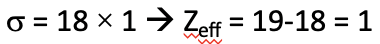
The net positive charge from the nucleus after accounting for shielding effects is called the effective nuclear charge. For the helium atom the effective nuclear charge is 1.34. We can calculate the effective nuclear charge from the experimentally measured first ionization energy. Solving the equation for Zeff gives Zeff=1.34 (Eq. 1.2.26).
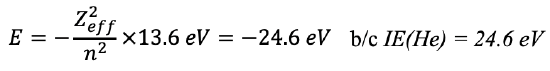

Equation 1.2.26 Calculation of Zeff in the Helium atom from first ionization energies.
The Lithium Atom
Now let us go to the atom with three electrons, the lithium atom. Following the so-called Aufbau principle we would fill the first two electrons into the 1s orbital, because the 1s orbital is the orbital with the the lowest energy. However, the third electron does not fit into the 1s orbital because of the Pauli principle.
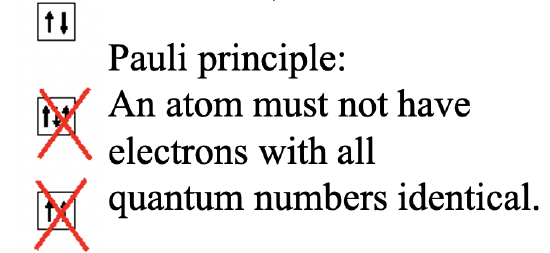
The Pauli principle states that no two electrons in an atom can have the same four quantum numbers. For that reason an orbital cannot accommodate more than two electrons. Within an orbital two electrons must have different spin quantum numbers s. We can indicate this by writing the electrons as arrows pointing up and down into a square box which represents the orbital. The third electron of the lithium would need to go to the orbital with the next higher energy.
According to the Schrödinger model, the energy of an orbital is only a function of the quantum number n, and we would have two choices: The 2s and the 2p orbitals. Both of them would have the same energy. However, in the lithium atom the 2s orbital has a somewhat lower energy than the 2p orbital. This can again be explained by shielding effects. The 2s orbital penetrates the 1s orbital slightly better than the 2p orbitals. Because of that, the 1s orbital shields the nuclear charge from the nucleus less for the 2s orbital compared to the 2p orbitals. The ground state electron configuration, which is the atom electron configuration having the lowest energy, must therefore be 1s2 2s1. We can see that the 2s orbital penetrates the 1s orbital slightly better than the 2p orbital from the graph for the radial probability functions of the orbitals shown in Figure 1.2.40.
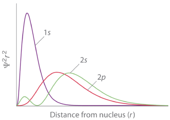
The second large maximum of the function of the 2s orbital is actually further away from the nucleus compared to the maximum associated with the 2p orbital. However, because the 2s orbital has a small second maximum very close to the nucleus, the 2s orbital overall penetrates the 1s orbital better, and therefore the shielding effect of the 1s orbital on the 2s orbital is smaller compared to the 2p orbitals.
Generally we can say, the smaller the quantum number l for a given quantum number n, the better the penetration ability of this orbital. Due to the better penetration ability, the shielding is less and thus the effective nuclear charge that acts on the electron in the orbital is higher. The higher effective nuclear charge leads to a lower energy of this orbital. For that reason the energy sequence of orbitals with the same quantum number n increases from s to p to d to f.
For example, a 3s orbital has a lower energy then a 3p orbital which has a lower energy than a 3d orbital (Fig. 1.2.41).
Slater's Rules
Because an orbital energy can be calculated from the effective nuclear charge, it would be useful if the effective nuclear charge could be somehow estimated by simple approximations.
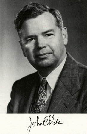
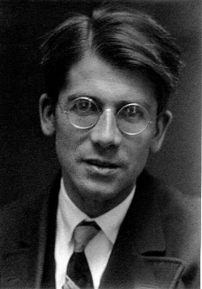
The so-called Slater rules, named after their developer John C. Slater (Fig. 1.2.42), are a simple tool that give a good estimate for the effective nuclear charge of orbitals in multi-electron atoms. The Slater rules estimate a shielding constant σ that allows to calculate the effective nuclear charge Zeff from the nuclear charge according to Zeff=Z-σ.
The rules for the estimation of σ are the following. Firstly, we need to recognize that the rules for s and p electrons are slightly different than those for d and f electrons. This is because s and p electrons of the same quantum number n have somewhat higher penetration abilities compared to d and f electrons. For both groups the first step is the same. We write out the electron configuration of the atom according to their quantum numbers n and l as shown below (Fig. 1.2.43).

Note that this order does not exactly reflect the order of energy. Electrons that have similar shielding effects are grouped together in parentheses. You can see that s and p orbitals of the same quantum number n build a group, all other orbitals are their own group.
To estimate the shielding constant for an s or a p orbital we can now apply the following rules:
a) Electrons to the right of the (ns, np) group contribute nothing to σ. This is because these electrons are further away from the nucleus than the electron of consideration.
b) Each of the other electrons in the same (ns, np) group contribute 0.35 to σ. These electrons are in the same shell as the electron of consideration, and thus have similar distance to the nucleus. For this reason their shielding is modest only and can be estimated to be about 35% of a full elementary charge, or 0.35.
c) Each electron in the n-1 shell contributes 0.85 to σ. Those electrons are significantly closer to the nucleus compared to the electron of consideration. For that reason they shield significantly better, approximately 85% of an elementary charge, or 0.85.
d) Each electron in the n-2 shell or below contributes 1.00 to σ. Those electrons are much closer to the nucleus than the electron of consideration and can fully shield an elementary charge. Its contribution to the shielding constant is therefore approximated to be 1.
Now let us look at the Slater rules for d and f electrons.
a) Electrons to the right of the (nd) or (nf) group contribute nothing to σ. This is again because the electron is further away from the nucleus than the electron of consideration, and thus cannot contribute to shielding.
b) Each of the other electrons in the same (nd) or (nf) group contribute 0.35 to σ. This is again because these electrons have similar distance compared to the electron for which we calculate the shielding constant, and thus the shielding is modest.
c) Each electron to the left of the (nd) or (nf) group contributes 1 to σ. Those electrons are considered much closer to the nucleus, and thus they shield a full elementary charge.
Note that the values 0.35, 0.85, and 1 have been chosen so that the results from the Slater rules are in the best possible accordance with experimental measurements of orbital energies. Remember, when we discussed the helium atom we said that the measurement of ionization energies can provide experimental orbital energies.
Slater's Rules Applied to Multi-Electron Atoms
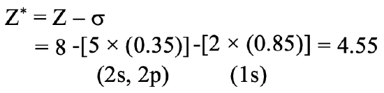
Let us practice the Slater rules by a few examples. We can, for instance, calculate the effective nuclear charge that acts on a 2p electron in an oxygen atom. To answer this question we need to first write out the electron configuration according to the quantum numbers n and l and group the orbitals correctly (Fig. 1.2.44).

Next, we need to consider that the effective nuclear charge Zeff is the nuclear charge Z minus the shielding constant σ. Then, because oxygen has eight protons, the nuclear charge is 8. From that we need to subtract the shielding constant. Firstly, we need to realize that there are 5 electrons in the same group as the 2p electron of consideration. These are the two 2s electrons and the three other 2p electrons. These five electrons shield with a factor of 0.35 because they are in the same group as the 2p electron for which we want to calculate the shielding constant. Note that this fourth 2p electron does not get a factor because it is the electron for which we calculate the shielding constant. In addition, we need to consider the two 1s electrons. They are in an n-1 shell, therefore they contribute with a factor of 0.85. Overall, the effective nuclear charge on the 2p electron is 8-(2 x 0.85)-(5 x 0.35)= 4.55 (Fig. 1.2.45).
We can also ask what is the effective nuclear charge on a 1s electron in the oxygen atom. It is 8-0.35=7.65 (Fig. 1.2.46).
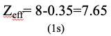
This is because we only need to consider the second electron in the 1s orbital to calculate the shielding constant σ. It contributes with a factor of 0.35 because it is in the same group as the 1s electron of consideration. The 2s and the 2p electrons are in a group right to the 1s orbital, therefore they do not contribute to the shielding.
Slater's Rules and the Aufbau Principle
The Slater rules are of great help to understand the so-called Aufbau principle, which says that for an atom in the ground state the electrons are in the orbitals of the lowest energy. To some extent the orbitals energies follow the quantum number n, but this is not always the case. For example, the element potassium has the electron configuration 1s2 2s2 2p6 3s2 3p6 3d0 4s1 and not 1s22s22p6 3s23p6 3d1. This means that the energy of the 3d orbital must be higher than the energy of the 4s orbital. Can the Slater rules predict that? Let us therefore calculate the energy of the 3d and 4s orbital using the Slater rules, and see if the energy of the 3d orbital comes out higher than the electron of the 4s orbital.
For the 3d orbital, the shielding constant is 18x1=18 because there are 18 electrons besides the 3d electron of consideration, and all the 18 electrons are in a lower shell. Therefore, they all contribute with a factor of 1. The nuclear charge Z of the potassium is 19. Therefore, the effective nuclear charge Zeff= 19-18=1 (Fig. 1.2.47).
Now let us do the analogous calculation for the 4s electron. For the 4s electron the Slater rules for s electrons apply. According to that, the two 3s and the six 3p electrons contribute 0.85 to the shielding constant because they are in an n-1 shell. The remaining two 1s, two 2s, and six 2p electrons are in an n-2 or lower shell and therefore contribute with the factor of 1. Therefore, the overall shielding constant is 8 x 0.85 + 10 x 1 = 16.8. The effective nuclear charge Zeff is therefore 19-16.8=2.2 (Fig. 1.2.48).

We can see that a higher effective nuclear charge acts on a 4s electron compared to a 3d electron, which indicates that the orbital energy for the 4s electron will be lower compared to the 3d electron. We can calculate the orbital energies by using the formula E=(Zeff2)/n2 ×13.6 eV (Eq. 1.2.27).
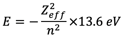
Equation 1.2.27 Equation for orbital energies
For the 3d electron we insert Zeff=1 and n=3 which gives -1.51 eV, Eq. 1.2.28.
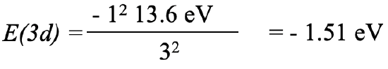
Equation 1.2.28 Equation for orbital energy of the 3d electron of potassium
For the 4s electron insert Zeff=2.2 and n=4 which gives -4.14 eV.
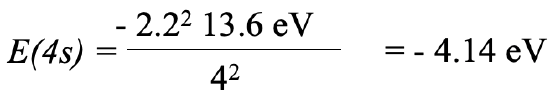
Equation 1.2.29 Equation for orbital energy of the 4s electron of potassium
As expected, the energy of the 4s electron is lower than the energy of the 3d electron. This explains why the electron configuration with the 4s electron as the valence electron is preferred over that with the 3d electron as the valence electron. Overall, we can see that the Slater rules can correctly predict electron configurations of atoms and the Aufbau principle.
Let us do another, more complex example: There are two conceivable electron configurations for Fe. One in which the 4s subshell is filled before the 3d subshell, and one in which the 3d subshell is filled before the 4s subshell. For the first case the electron configuration is 1s22s22p63s2 3p6 4s2 3d6. For the second case, the second electron configuration is 1s2 2s2 2p6 3s2 3p6 3d8 4s0. We can see that the two electron configurations are the same for the 1s, 2s, 2p, 3s, and 3p electrons. We therefore focus on the remaining eight electrons, denoted in red, and calculate their energies.
In this case, we need to compare the sum of the electron energies for both electron configurations to be able to decide which electron configuration is favored. We calculate the sum of the energies of the eight electrons for the first electron configuration the following way: In the first step we need to rewrite the electron configuration in Slater form: (1s2)(2s2 2p6)(3s2 3p6)(3d6)(4s2).
Next, we can calculate the shielding constant for a 3d electron. We can ignore the two 4s electrons because they are to the right of the d electron of consideration, and do not contribute to the shielding. However, we do need to consider the five other 3d electrons that are in the same group as the 3d electron of consideration. They contribute with the factor of 0.35. The other 18 electrons contribute 1.00 because they are in a lower shell. Because the effective nuclear charge of Fe is 26, the effective nuclear charge Zeff is Zeff=26-19.75=6.25 (Eq. 1.2.30).

Equation 1.2.30 Equation for the shielding constant and effective nuclear charge of the 3d electron of an iron atom
For a 4s electron, there is one other 4s electron in the same group which contributes with a factor of 0.35. In addition, there are 14 electrons in an n-1 shell, namely the 3s, the 3p, and the 3d electrons. They contribute 0.85 to the shielding constant. The remaining 10 electrons are in an n-2 shell or lower, therefore they contribute with the factor 1.00. This gives an overall shielding constant of 22.25. From that we can calculate the effective nuclear charge for a 4s electron which is 26-22.25=3.75.

Equation 1.2.31 Equation for shielding constant and effective nuclear charge of the 4s electron of an Fe atom
We can now calculate the electron energies. It is the sum of the energies for the 3d and 4s electrons. The electron energy for a single electron is E=-(Zeff2)/n2 ×13.6 eV= -(6.252)/32×13.6 eV=-59.03 eV. Because we have six 3d electrons, the overall energy for the six electrons is 6 x -59.03 eV = -354.17 eV (Eq. 1.2.32).
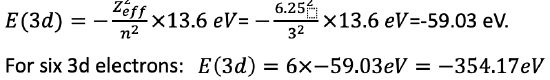
Equation 1.2.32 Equation for the electron energies of the six 3d electrons in an iron atom
The energy of a single 4s electron is E=-(3.752)/42 ×13.6 eV=-11.95 eV. For two 4s electrons the energy is 2 x -11.95 eV= -23.90 eV.
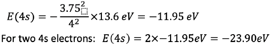
Equation 1.2.33 Equation for the electron energies of the 4s electron in iron
The sum of all electrons is then -354.17 eV + (-23.90 eV) = -378.1 eV (Eq. 1.2.34).

Equation 1.2.34 Equation for the sum of all electrons
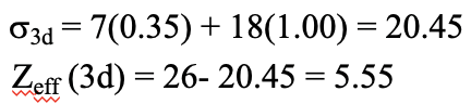
Now let us calculate the energy for the second electron configuration. First we need this electron configuration in Slater configuration. Next, we can calculate the shielding constant for the d electrons. It is σ3d = 7(0.35) + 18(1.00) = 20.45 because there are seven other 3d electrons in the same group and 18 electrons in lower shells. The effective nuclear charge is then Zeff (3d) = 26- 20.45 = 5.55.
Equation 1.2.35 Equation for the shielding constant and effective nuclear charge of the 3d electrons of iron (second configuration)
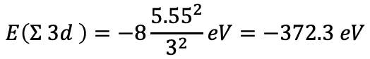
The sum of the electron energies for the eight d electrons is then E(Σ 3d)=-8(5.552/32 ) eV=-372.3 eV, Eq. 1.2.36.
Equation 1.2.36 Equation for the sum of the electron energies for the eight d electrons of iron
We can can see the energy of the second electron configuration is somewhat higher, and thus less preferred. This is in accordance with the experimentally observed ground state electron configuration of the Fe atom. Again, we see that the Slater rules can correctly predict the ground state electron configuration of atoms.
The Aufbau Principle and the Spin Pairing Energy
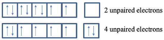
The Slater rules are suitable to account for shielding effects in multi-electron atoms which are of electrostatic nature. However, not only electrostatic effects influence the orbital energies, there are also magnetic effects. This is because each electron has a spin with a magnetic field associated with it. The electrons behave like little magnets that can interact with each other. These interactions can be either attractive or repulsive, which influences the electron energies. The electron energies are usually minimized when the number of electrons with the same spin is maximized. This is known as Hund’s (Fig. 1.2.49) rule of maximum spin multiplicity.
In the previously example we have seen that the electron configuration 4s2 3d6 is favored in Fe because of electrostatic shielding effects. In addition, it also favored by magnetic effects. In this electron configuration there are four unpaired electrons, while in the electron configuration 3d8 there are only two unpaired electrons.
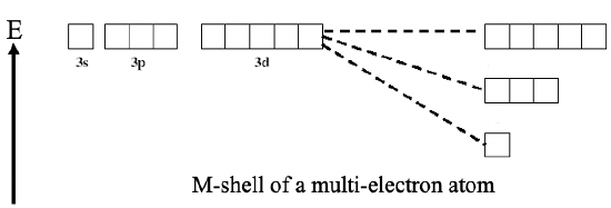
We can now understand the Aufbau principle for multi-electron atoms (Figure 1.2.51).
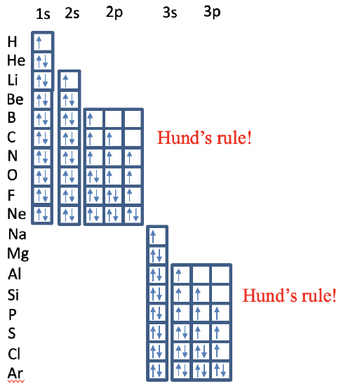
For H and He the 1s orbital gets filled. From lithium to beryllium the 2s subshell gets filled, and from boron to neon the 2p subshell gets filled under consideration of Hund's rule. You can see that for carbon the two 2p electrons are both spin up in different 2p orbitals. For nitrogen there are three unpaired electrons in the 2p orbitals. From the element oxygen on, we have to start pairing spins until all spins are paired in neon. From Na to Ar the 3s and the 3p orbitals get filled according to the same principles.
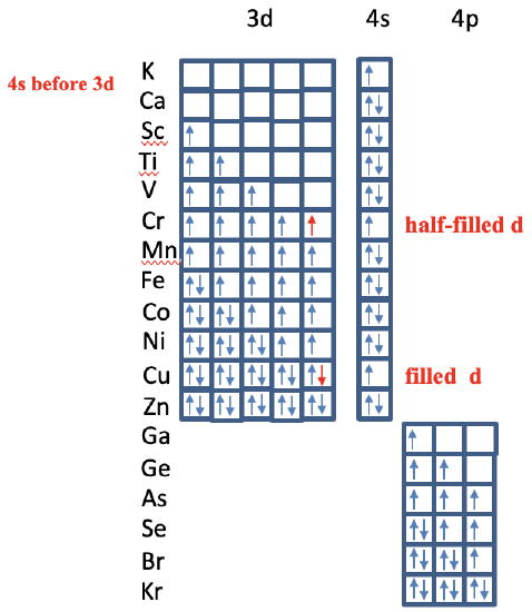
After that, the 4s orbitals of K and Ca get filled, and then the 3d orbitals of the elements from Sc to Zn (Fig. 1.2.52). We have seen previously that the Slater rules nicely show why. You can see that there are two anomalies though. For the chromium, the electron configuration is 4s1 3d5 and not 4s2 3d4. This is because there are more unpaired spins in this electron configuration, and a half-filled 3d subshell with unpaired spins only represents a particularly stable electron configuration. The second anomaly occurs for the element Cu which has an electron configuration 4s13d10 and not 4s23d9. This is because a d10 electron configuration is a particular stable electron configuration. After the 3d subshell is filled, the 4p subshell is filled for the elements from Ga to Kr. Again, the electrons are filled into the orbitals according to Hund’s rule. We could extend our consideration to even heavier elements, but will be beyond scope.
Dr. Kai Landskron (Lehigh University). If you like this textbook, please consider to make a donation to support the author's research at Lehigh University: Click Here to Donate.