3.12: Electronic Structure and the Periodic Table
- Page ID
- 221341
Learning Objectives
- Relate the electron configurations of the elements to the shape of the periodic table.
- Determine the expected electron configuration of an element by its place on the periodic table.
- Predict group and period for an element given its electron configuration
In Chapter 2, we introduced the periodic table as a tool for organizing the known chemical elements. A periodic table is shown in Figure \(\PageIndex{1}\). The elements are listed by atomic number (the number of protons in the nucleus), and elements with similar chemical properties are grouped together in columns.
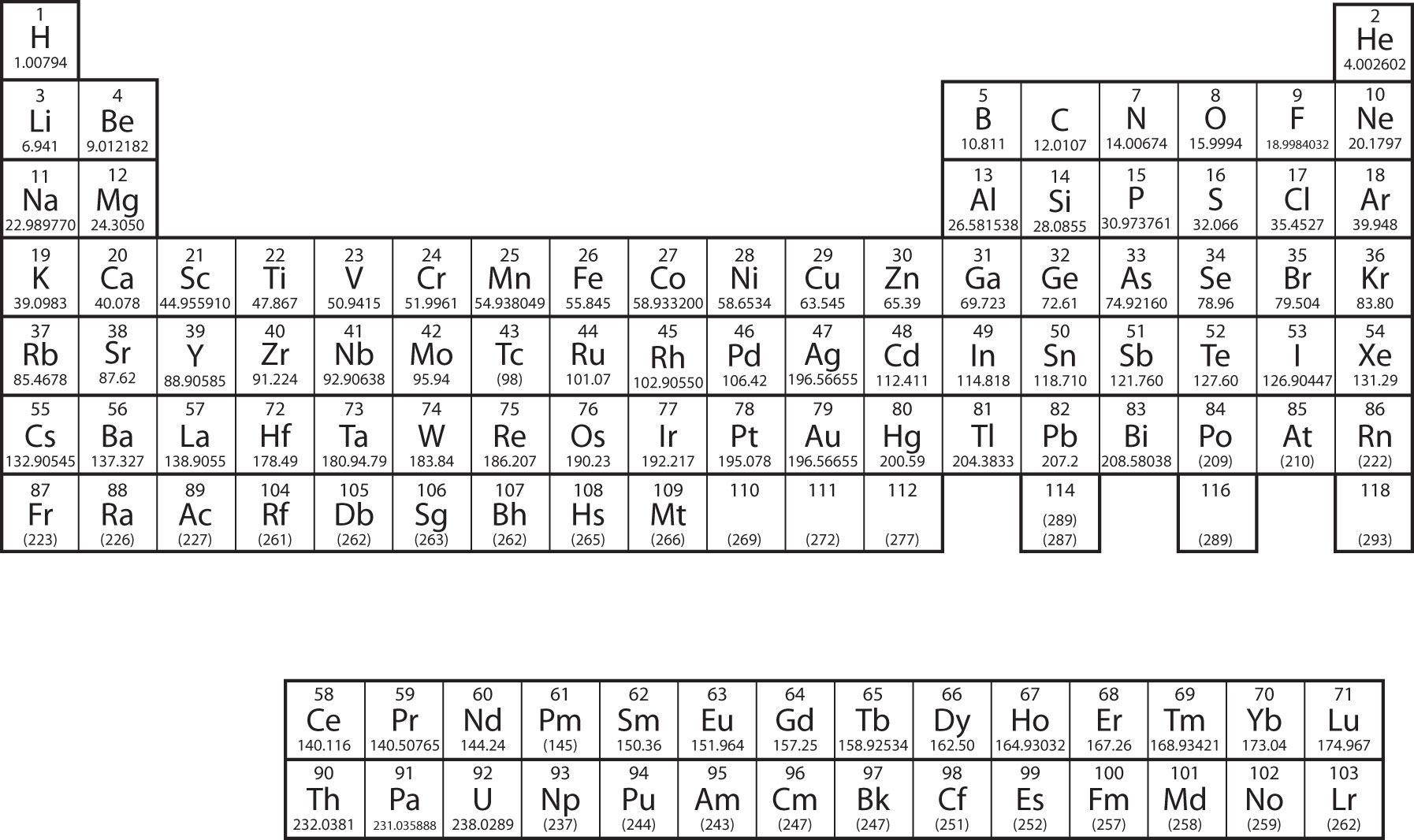
Why does the periodic table have the structure it does? The answer is rather simple, if you understand electron configurations, the shape of the periodic table mimics the filling of the subshells with electrons.
The shape of the periodic table mimics the filling of the subshells with electrons.
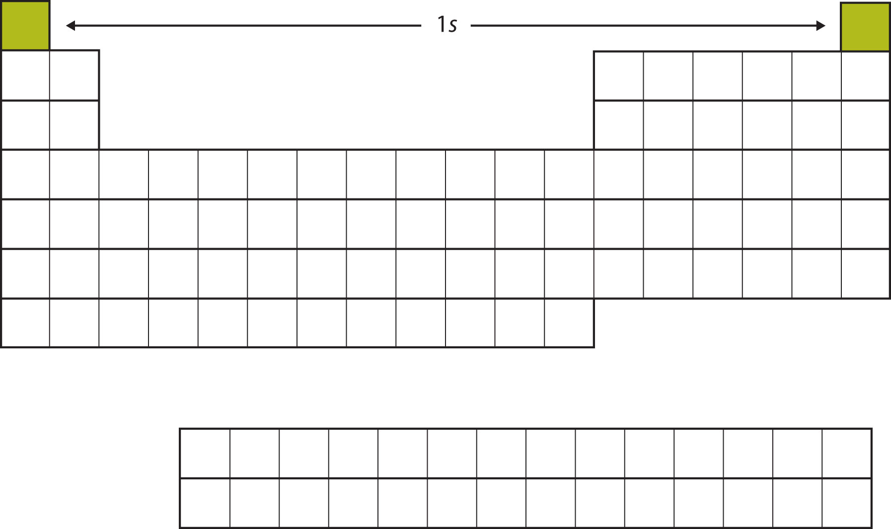
Let us start with H and He. Their electron configurations are 1s1 and 1s2, respectively; with He, the n = 1 shell is filled. These two elements make up the first row of the periodic table (Figure \(\PageIndex{2}\))
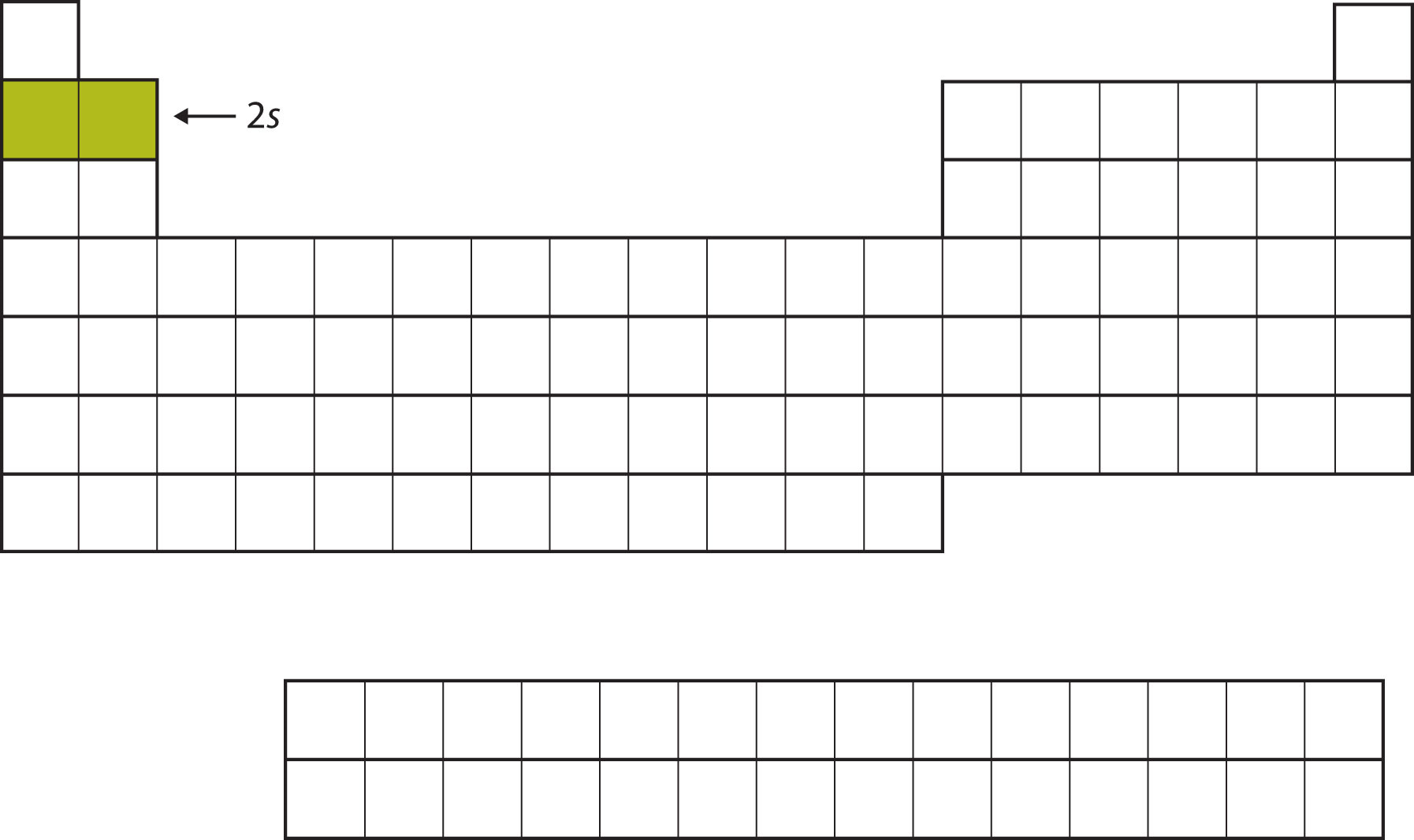
The next two electrons, for Li and Be, would go into the 2s subshell. Figure \(\PageIndex{3}\) shows that these two elements are adjacent on the periodic table.
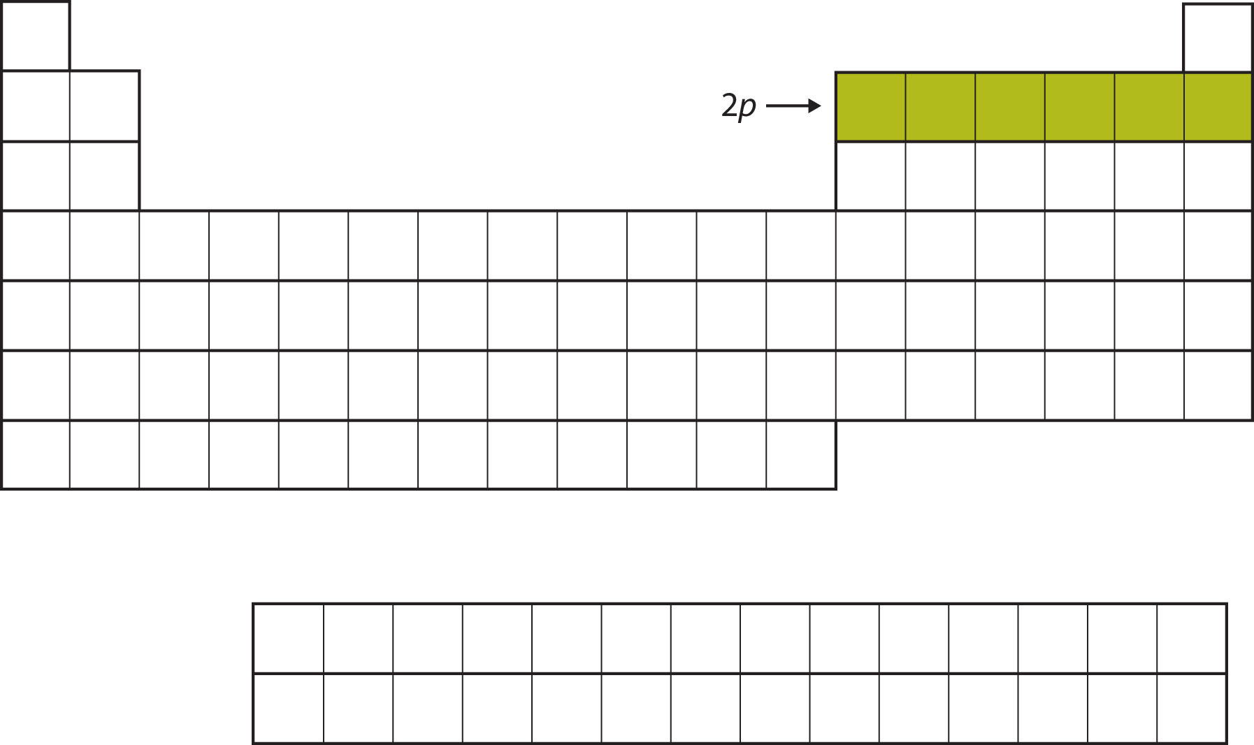
For the next six elements, the 2p subshell is being occupied with electrons. On the right side of the periodic table, these six elements (B through Ne) are grouped together (Figure \(\PageIndex{4}\)).
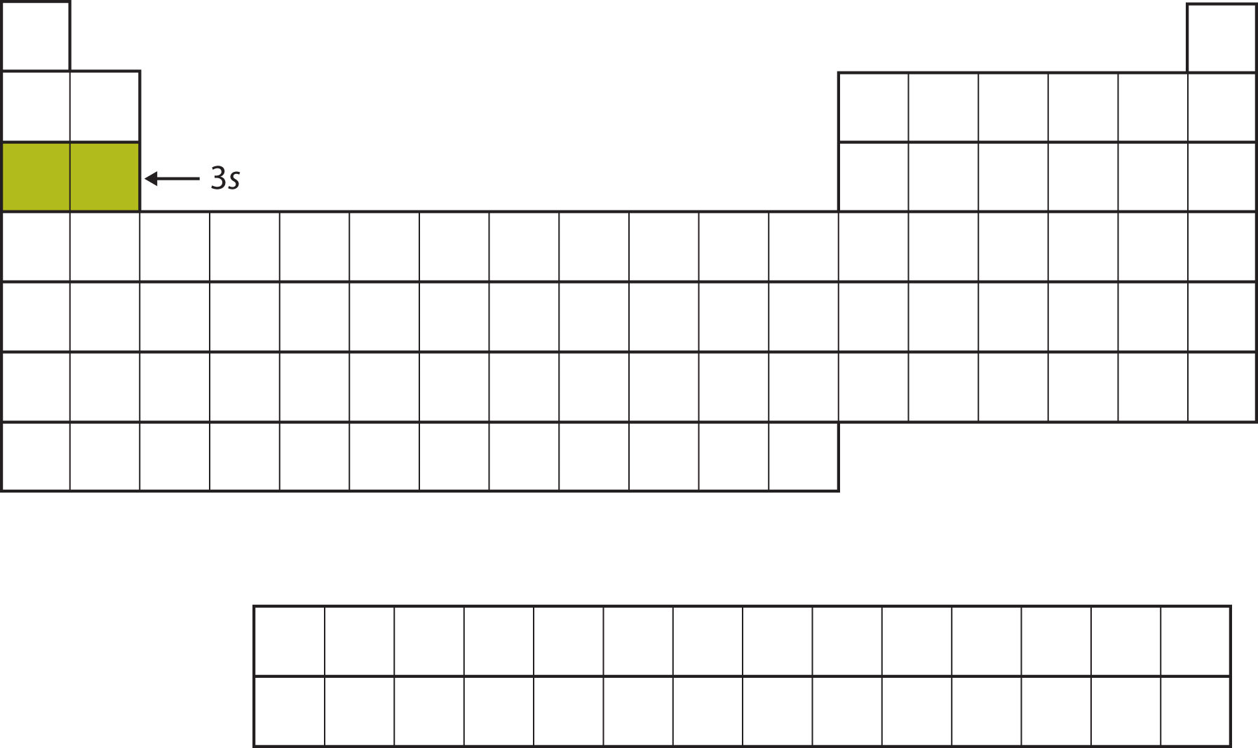
The next subshell to be filled is the 3s subshell. The elements coinciding this subshell being filled, Na and Mg, are back on the left side of the periodic table (Figure \(\PageIndex{5}\)).
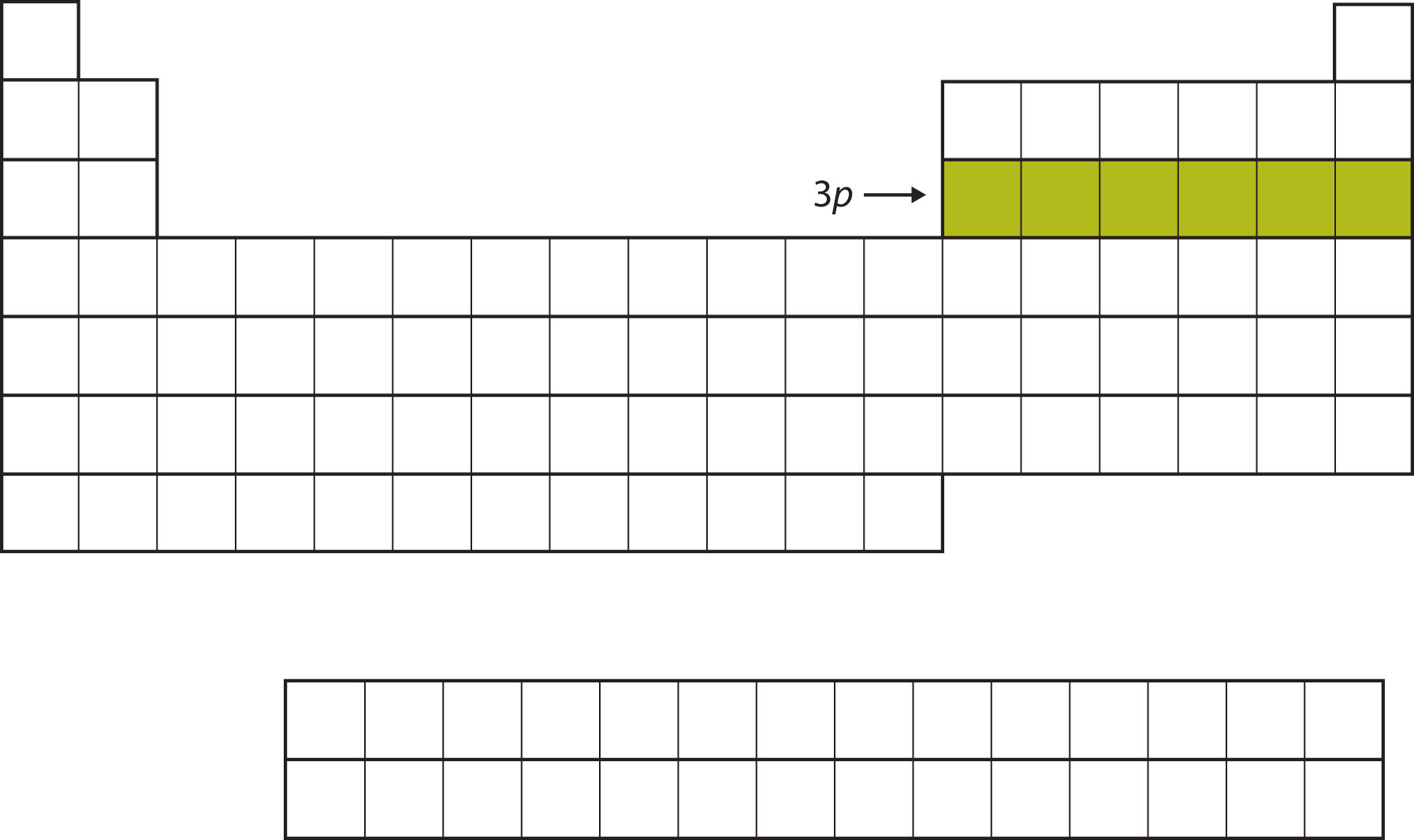
Next, the 3p subshell is filled with the next six elements (Figure \(\PageIndex{6}\)).
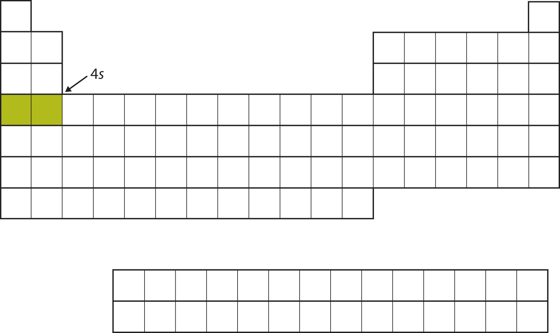
Instead of filling the 3d subshell next, electrons go into the 4s subshell (Figure \(\PageIndex{7}\)).
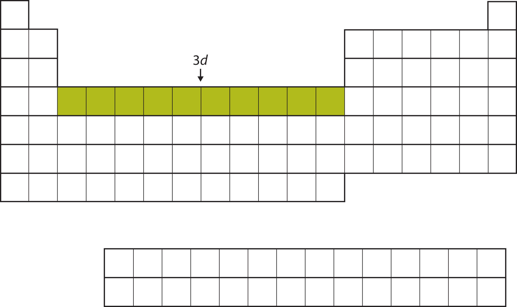
After the 4s subshell is filled, the 3d subshell is filled with up to 10 electrons. This explains the section of 10 elements in the middle of the periodic table (Figure \(\PageIndex{8}\)).
And so forth. As we go across the columns of the periodic table, the overall shape of the table outlines how the electrons are occupying the shells and subshells.
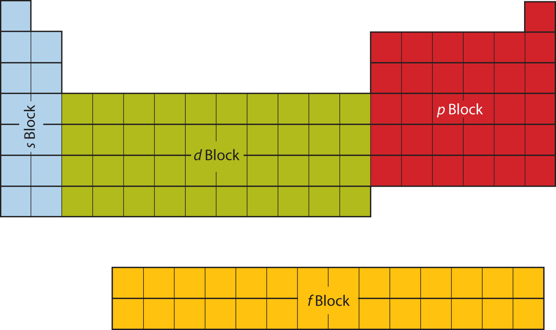
The first two columns on the left side of the periodic table are where the s subshells are being occupied. Because of this, the first two rows of the periodic table are labeled the s block. Similarly, the p block is the right-most six columns of the periodic table, the d block is the middle 10 columns of the periodic table, while the f block is the 14-column section that is normally depicted as detached from the main body of the periodic table. It could be part of the main body, but then the periodic table would be rather long and cumbersome. Figure \(\PageIndex{9}\) shows the blocks of the periodic table.
The electrons in the highest-numbered shell, plus any electrons in the last unfilled subshell, are called valence electrons; the highest-numbered shell is called the valence shell. (The inner electrons are called core electrons.) The valence electrons largely control the chemistry of an atom. If we look at just the valence shell's electron configuration, we find that in each column, the valence shell's electron configuration is the same. For example, take the elements in the first column of the periodic table: H, Li, Na, K, Rb, and Cs. Their electron configurations (abbreviated for the larger atoms) are as follows, with the valence shell electron configuration highlighted:
| H: | 1s1 |
| Li: | 1s22s1 |
| Na: | [Ne]3s1 |
| K: | [Ar]4s1 |
| Rb: | [Kr]5s1 |
| Cs: | [Xe]6s1 |
They all have a similar electron configuration in their valence shells: a single s electron. Because much of the chemistry of an element is influenced by valence electrons, we would expect that these elements would have similar chemistry—and they do. The organization of electrons in atoms explains not only the shape of the periodic table, but also the fact that elements in the same column of the periodic table have similar chemistry.
The same concept applies to the other columns of the periodic table. Elements in each column have the same valence shell electron configurations, and the elements have some similar chemical properties. This is strictly true for all elements in the s and p blocks. In the d and f blocks, because there are exceptions to the order of filling of subshells with electrons, similar valence shells are not absolute in these blocks. However, many similarities do exist in these blocks, so a similarity in chemical properties is expected.
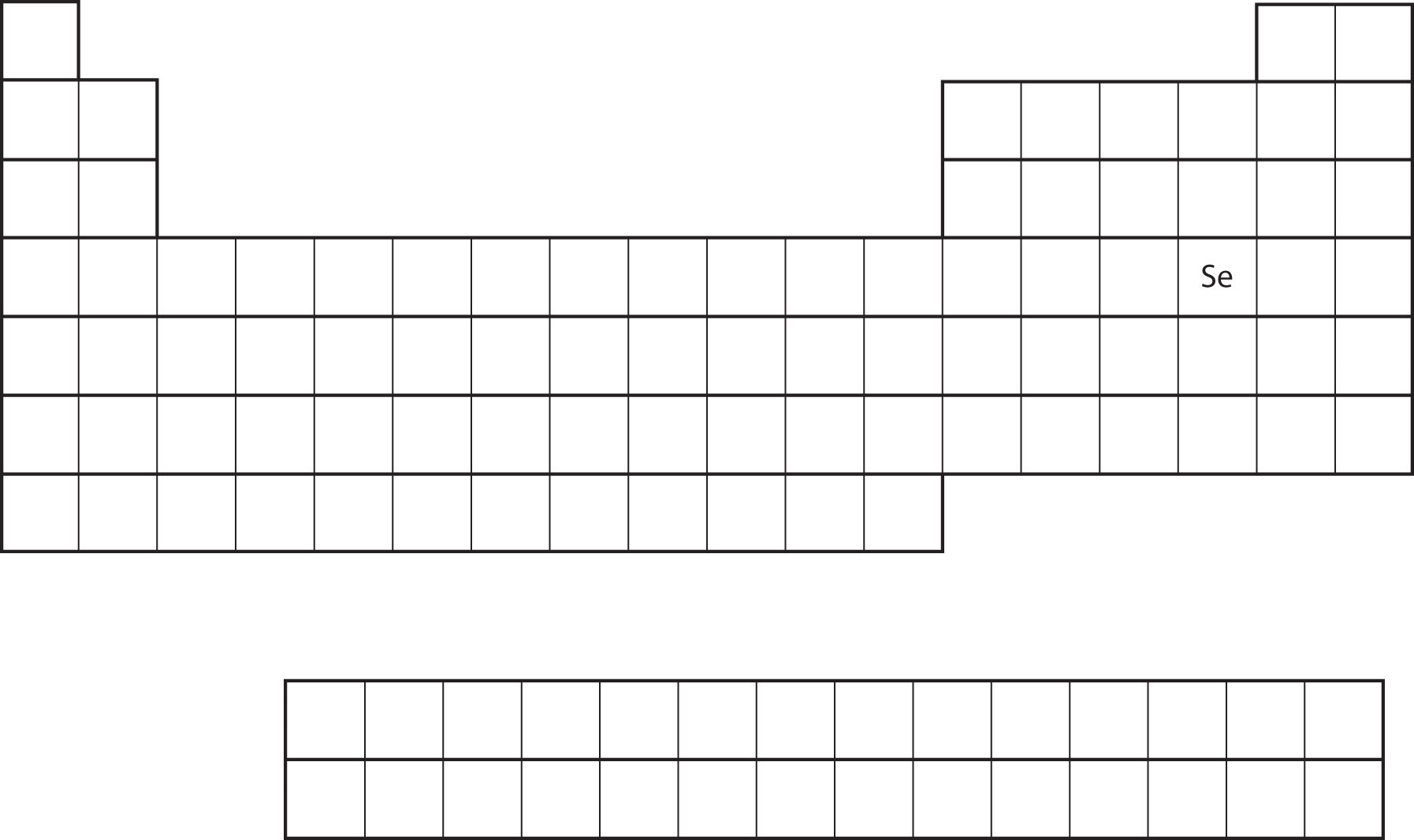
Similarity of valence shell electron configuration implies that we can determine the electron configuration of an atom solely by its position on the periodic table. Consider Se, as shown in Figure \(\PageIndex{10}\). It is in the fourth column of the p block. This means that its electron configuration should end in a p4 electron configuration. Indeed, the electron configuration of Se is [Ar]4s23d104p4, as expected.
Example \(\PageIndex{1}\):
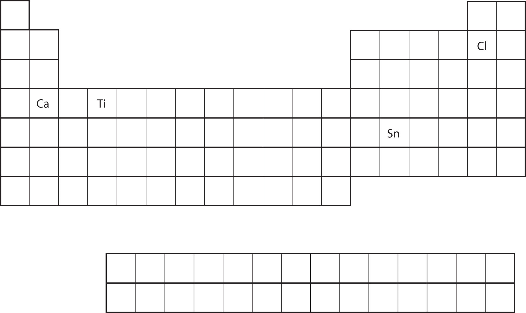
From the element's position on the periodic table, predict the valence shell electron configuration for each atom (Figure \(\PageIndex{11}\)).
- Ca
- Sn
Solution
- Ca is located in the second column of the s block. We would expect that its electron configuration should end with s2. Calcium's electron configuration is [Ar]4s2.
- Sn is located in the second column of the p block, so we expect that its electron configuration would end in p2. Tin's electron configuration is [Kr]5s24d105p2.
Exercise \(\PageIndex{1}\)
From the element's position on the periodic table, predict the valence shell electron configuration for each atom. Figure \(\PageIndex{11}\).
- Ti
- Cl
- Answer a
-
[Ar]4s23d2
- Answer b
-
[Ne]3s23p5
Food and Drink Application: Artificial Colors
The color of objects comes from a different mechanism than the colors of neon and other discharge lights. Although colored lights produce their colors, objects are colored because they preferentially reflect a certain color from the white light that shines on them. A red tomato, for example, is bright red because it reflects red light while absorbing all the other colors of the rainbow.
Many foods, such as tomatoes, are highly colored; in fact, the common statement "you eat with your eyes first" is an implicit recognition that the visual appeal of food is just as important as its taste. But what about processed foods?
Many processed foods have food colorings added to them. There are two types of food colorings: natural and artificial. Natural food colorings include caramelized sugar for brown; annatto, turmeric, and saffron for various shades of orange or yellow; betanin from beets for purple; and even carmine, a deep red dye that is extracted from the cochineal, a small insect that is a parasite on cacti in Central and South America. (That's right—you may be eating bug juice!)
Some colorings are artificial. In the United States, the Food and Drug Administration currently approves only seven compounds as artificial colorings in food, beverages, and cosmetics:
- FD&C Blue #1: Brilliant Blue FCF
- FD&C Blue #2: Indigotine
- FD&C Green #3: Fast Green FCF
- RD&C Red #3: Erythrosine
- FD&C Red #40: Allura Red AC
- FD&C Yellow #5: Tartrazine
- FD&C Yellow #6: Sunset Yellow FCF
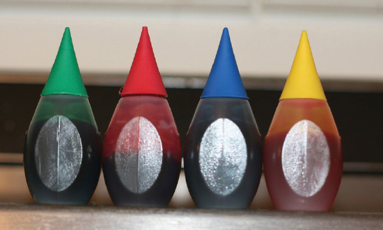
Lower-numbered colors are no longer on the market or have been removed for various reasons. Typically, these artificial colorings are large molecules that absorb certain colors of light very strongly, making them useful even at very low concentrations in foods and cosmetics. Even at such low amounts, some critics claim that a small portion of the population (especially children) is sensitive to artificial colorings and urge that their use be curtailed or halted. However, formal studies of artificial colorings and their effects on behavior have been inconclusive or contradictory. Many people continue to enjoy processed foods with artificial coloring (like those shown in the accompanying figure).
Predicting group and period from the electron configuration
As you can imagine from our discussion above, there is a clear connection between electron configuration and location on the periodic table. We might ask ourselves if there is a simple way to predict the group and period for an element given its electron configuration. The answer is yes, we just need to consider the valence electrons for that element to be able to predict its location on the periodic table. The general rule is that the period for an element is the same as the highest occupied electron shell (n) for that element, while the group corresponds to the total number of valence electrons. In the case of valence electrons with p-type orbital, we need to add 10 to the number of valence electrons in order to determine the group in the 1-18 group system. Examples:
-
Lithium has an electron configuration 1s2 2s1. The highest occupied electron shell is 2, so the period number is 2. The number of valence electrons is 1 (no p-valence electrons), so the group number is 1.
-
Boron has an electron configuration 1s2 2s2 2p1. The highest occupied electron shell is 2, so the period number is 2. The number of valence electrons is 3, but they include electrons in a p-type orbital, so to calculate the group number we need to add 10 to the number of valence electrons. So group number= 10 + 3 = 13.
-
Iron has an electron configuration 1s2 2s2 2p6 3s2 3p6 4s2 3d6. The highest occupied electron shell is 4, so the period number is 4. The number of valence electrons is 8 (no p-valence electrons), so the group number is 8.
Summary
The arrangement of electrons in atoms is responsible for the shape of the periodic table. Electron configurations can be predicted by the position of an atom on the periodic table.

