3.9B: Particle in a Finite Box and Tunneling (optional)

The finite potential well is an extension of the infinite potential well from the previous section. The main difference between these two systems is that now the particle has a non-zero probability of finding itself outside the well, although its kinetic energy is less than that required, according to classical mechanics, for scaling the potential barrier [4]. This type of problem is more realistic, but more difficult to solve due to the yielding of transcendental equations. The particle is again confined to a box, but one which has finite, not infinite, potential walls. We consider a potential well of height V0.

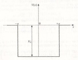
Figure 2.1 Square well with finite potential. Here, a=L.

We have the following potential, V(x), given by the boundary conditions shown in Figure 2.1:

In this example, the origin of the x-axis was chosen at the center of the well. By doing so, the potential is symmetric about x=0, giving rise to parity (Note: this could also be applied to a symmetric infinite wells). For the finite well, two cases must be distinguished, corresponding to positive or negative values of the energy E [1]. It is possible for the particle to be bound, or unbound. The case E<0 corresponds to a particle which is confined (and whose energy is less than the well depth) and hence is in a bound state [1]. When E>0, the particle is unconfined and corresponds to a scattering problem. The latter case will only briefly be discussed.

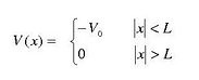
Figure 2.2 [7] provides a prelude to what the wavefunctions and probability distributions for several states will look like in a finite well. Comparing Figure 2.2 with Figure 1.2 for the infinite case, we see that in the finite case, the wavefunctions do not have to be zero at the walls of the well. In the finite case, the wavelengths are slightly longer, implying that the allowed energies will be somewhat smaller.

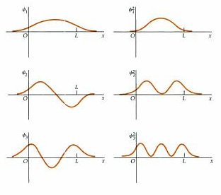
Figure 2.2 In this figure, the points O and L represent the walls of the well.

Case 1: Bound State

In the bound state we have,−V0<=E<0 (since E cannot be lower than the absolute minimum of the potential [1]. The Schrodinger equation for the two regions is given by [6]

Here, the binding energy, |E| of the particle is introduced (|E|=−E). To simplify the TISE equations, let,

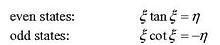
The solutions of the TISE separate into even and odd parity states, and we need only consider positive values of x (which could be inferred from the potential). With the application of the boundary conditions, the even solutions are given as [6]

and the odd solutions are given as [1]

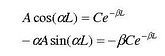
Despite the discontinuous nature of the potential at x=L, the wavefunction and its derivative are still continuous, and these conditions provide the required boundary conditions to determine the quantized energies [6]. The requirements that ψO=psiE(x) and Missing open brace for superscript? yields the two equations

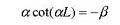
These can be combined to give the even eigenvalue condition (which depends on the energies but not on the constants A and C) [6] is

The odd eigenvalue condition is found to be

The energy levels of the bound states are found by solving these transcendental equations, either graphically or numerically [1]. In doing so, it is helpful to change to dimensionless variables. We introduce the dimensionless quantities [1]

Upon substitution these quantities, the transcendental equations become

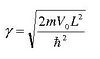
The graphical determination of the energy levels are obtained by finding the points of intersection of the circle (See Graph 2.1)[1]

where γ is of known radius (found by simple substitution),

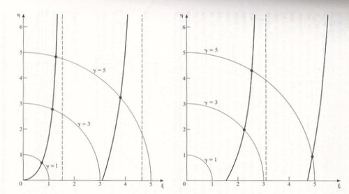
Graph 2.1.1 The left graph shows energy levels for even states, while the right graph represents odd states.

What can be concluded from this figure?

• The bound-state energy levels are non-degenerate.
• The bound-state energy levels are finite, but increase without bound and depend on the parameter γ. Thus, deeper and wider potentials have a larger number of bound states.
• The bound state spectrum consists of alternating even and odd states, with the ground state always being even.

Case 2: Unbound State

The finite well problem shows that wavefunctions are not localized in the vicinity of the well[10] . This is the case of unbound states, where eigenvalues of energy are a continuum. In this problem, a particle is incident upon the well from the left, interacts with the well, and gets transmitted or reflected. The solution of the Schrodinger equation is outlined briefly. Note that in one dimension, there is a lack of symmetry between the external regions to the left and right of the potential, since the particle is assumed to be incident on the potential in a given direction [6]. Therefore, there is no need to exercise parity.

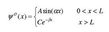
For the external regions, the solution of the TISE is given by [1]

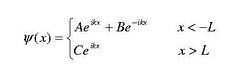
where

In the region of x<−L, the wavefunction is seen to consist of an incident wave of amplitude A and a reflected wave of amplitude B. In the region of x>L, the wavefunction is seen as a pure transmitted wave of amplitude C [1].

For the internal region, the solution of the TISE is given by [1]

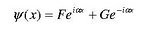
where,

By applying continuity at x=L and x=−L, F and G are eliminated and the ratios of B/A and C/A can be solved to obtain the reflection coefficient, R=|B/A|2, and the transmission coefficient, T=|C/A|2. An important aspect to briefly point out is that the transmission coefficient is generally less than unity, which is in contradiction to the classical prediction that suggests that the particle should always be transmitted

Summary

To summarize, the major differences between a particle in a finite box and an infinite well, are [((web1))]:

• Only a finite number of energy levels exist (bound state)
• Tunneling into the barrier (wall) is possible
• Higher energy states are less tightly bound than lower ones
• A particle provided with enough energy can escape the well (unbound state)

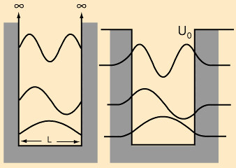
Figure 2.2.1 Comparison of infinite and finite well.

We have considered in some detail a particle trapped between infinitely high walls a distance L apart, we have found the wavefunction solutions of the time independent Schrödinger equation, and the corresponding energies. The essential point was that the wavefunction had to go to zero at the walls, because there is zero probability of finding the particle penetrating an infinitely high wall. This meant that the lowest energy state couldn't have zero energy, that would give a constant nonzero wavefunction. Rather, the lowest energy state had to have the minimal amount of bending of the wavefunction necessary for it to be zero at the two walls but nonzero in between-this corresponds to half a period of a sine or cosine (depending on the choice of origin), these functions being the solutions of Schrödinger's equation in the zero potential region between the walls. The sequence of wavefunctions (eigenstates) as the energy increases have 0, 1, 2, … zeros (nodes) in the well.

Let us now consider how this picture is changed if the potential at the walls is not infinite. It will turn out to be convenient to have the origin at the center of the well, so we take

• \(V(x) = V_0 \) for \(x < -L/2\)
• \(V(x) = 0\) for \(-L/2 < x < L/2\)
• \(V(x) = V_0\) for \(L/2 < x\).

Having the potential symmetric about the origin makes it easier to catalog the wavefunctions. For a symmetric potential, the wavefunctions can always be taken to be symmetric or antisymmetric.

Symmetry

If a wavefunction \(ψ(x)\) is a solution of Schrödinger's equation with energy \(E\), and the potential is symmetric, then \(ψ(-x)\) is a solution with the same energy. This means that \(ψ(x)+ ψ(-x)\) and \(ψ(x)- ψ(-x)\) are also solutions, since the equation is linear, and these are symmetric and antisymmetric respectively, and using them is completely equivalent to using the original \(ψ(x)\) and its reflection \(ψ(-x)\).

How is the lowest energy state wavefunction affected by having finite instead of infinite walls? Inside the well, the solution to Schrödinger's equation is still of cosine form (it's a state symmetric about the origin). However, since the walls are now finite, ψ(x) cannot change slope discontinuously to a flat line at the walls. It must instead connect smoothly with a function which is a solution to Schrödinger's equation inside the wall.

The equation in the wall is

\[ \dfrac{-\hbar^2}{2m} \dfrac{d^2 \psi(x)}{dx^2} + V_0 \psi(x) = E(x)\]

and has two exponential solutions (say, for \(x > L/2\)) one increasing to the right, the other decreasing,

\(e^{\alpha x}\) and \(e^{- \alpha x}\)

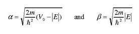
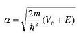
where

\[\alpha = \sqrt{2m(V_o-E)/hbar^2}\]

(We are assuming here that \(E < V_0\), so the particle is bound to the well. We shall find this is always true for the lowest energy state.)

Let us try to construct the wavefunction for the energy E corresponding to this lowest bound state. From the equation with \(V_0 = 0\), the wavefunction inside the well (let's assume it's symmetric for now) is proportional to \(\cos kx\), where \(k= \sqrt{2mE/\hbar^2}\).

The wavefunction (and its derivative!) inside the well must match a sum of exponential terms—the wavefunction in the wall—at \(x = L/2\), so

\[ \cos \left(\dfrac{kL}{2} \right) = A e^{\alpha L/2} + B e^{- \alpha L/2} \]

\[ -k \sin \left(\dfrac{kL}{2} \right) = \alpha e^{\alpha L/2} -\alpha e^{- \alpha L/2} \]

(By writing just a cosine term inside the well, we have left out the overall normalization constant. This can be put back in at the end.)

Solving these equations for the coefficients \(A\), \(B\) in the usual way, we find that in general the cosine solution inside the well goes smoothly into a linear combination of exponentially increasing and decreasing terms in the wall. (By the symmetry of the problem, the same thing must happen for x < -L/2.) However, this cannot in general represent a bound state in the well. The increasing solution increases without limit as \(x\) goes to infinity, so since the square of the wavefunction is proportional to the probability of finding the particle at any point, the particle is infinitely more likely to be found at infinity than anywhere else. It got away! This clearly makes no sense—we're trying to find wavefunctions for particles that stay in, or at least close to, the well. We are forced to conclude that the only exponential wavefunction that makes sense is the one for which A is exactly zero, so that there is only a decreasing wave in the wall.

Requiring the decreasing wavefunction, \(A = 0\), means that only a discrete set of values of \(k\), or \(E\), satisfy the boundary condition equations above. They are most simply found by taking \(A = 0\) and dividing one equation by the other to give:

\[ \tan \left(\dfrac{kL}{2} \right) = \dfrac{\alpha}{k}\]

This cannot be solved analytically, but is easy to solve graphically by plotting the two sides as functions of \(k\) and finding where the curves intersect.

Using the Spreadsheet for the Finite Square Well

Recall that by taking the origin in the center of the square well, we argued that we need only look at wavefunctions that were symmetric or antisymmetric about the origin. If you try to sketch such wavefunctions, you will find that symmetric wavefunctions must have zero slope at the origin, and antisymmetric wavefunctions must be zero at the origin.

Furthermore, if we know the wavefunction in the right-hand half, that is, for x > 0, we know it for all x, from the symmetry. Hence, we need only solve Schrödinger's equation going from the origin to the right - we can take x₀ = 0, x₁ = dx, etc.

As we discussed in the preceding section, on integrating out from the origin with energy E set less than V₀, once we cross over into the wall the solution is some combination of an exponentially increasing function and an exponentially decreasing function,

where the exponential coefficient α is positive, and depends on E—it was defined in the preceding section.

Let us first look at the symmetric solutions for very low energies, so take f(0) = 1, f'(0) =0. (Note that we cannot find the correct overall normalization constant until we find the solution, then integrate its square over all space—this can always be done later, and is unnecessary for analyzing the properties of the state).

Let us begin with the trivial case E = 0. For zero energy, inside the well E - V will of course be identically zero, so from Schrödinger's equation the slope of f(x) can never change, consequently f(x) = 1 for all x < L. On reaching the wall, this wavefunction and its derivative connect smoothly from inside to outside if A = B = ½. It is clear that as we keep going to the right, the A term in the above equation dominates and f(x) diverges, signaling that there is no state localized in the well at E = 0.

At this point, you should create an Excel spreadsheet, with a graph showing f(x) and V(x)-E as functions of x. Details of how this might be done are given in the accompanying homework assignment. If you have a working spreadsheet, it will be much easier to understand the following discussion!

As we now increase E from zero, the symmetric wavefunction, having zero slope at the center of the well, will begin to curve downwards on moving away from the center, and as the energy increases so does the downward curvature. This naturally changes the mix of increasing and decreasing exponentials needed to connect smoothly at the wall, and in fact as a function of E, A(E) changes sign at a certain value we will call E₀. For energies just below E₀, f(x) diverges to plus infinity for large x. For energies above E₀, it diverges to minus infinity for large x. Exactly at E₀, f(x) goes to zero for large x. This is the wavefunction we are looking for: it corresponds to a particle localized close to the well, and in fact is the lowest possible energy—the ground state—for a particle in the well. E₀ is called the ground state eigenvalue, the wavefunction is called an eigenstate.

Finding the Ground State Energy

The first problem is to find this value E₀. If we just guess a value of E, the wavefunction will almost certainly diverge for large x. The way to find E₀ is to notice that for E below E₀, f(x) goes to large positive values on the far right, for E just above E₀, f(x) goes to large negative values on the far right. So we take an increasing set of E values starting near zero, and watch for the tail to wag! When this happens, we back up half way, then back or forward as necessary, choosing a set of E values that bracket E₀.

Actually, this rather tedious process can be automated in Excel, but it's worth going through it manually a time or two to get a feeling for how the wavefunctions behave. A general feature to check is that for E > V(x) they are oscillatory, sine or cosine like, although with changing wavelengths in general; whereas for E < V(x) they have exponential character. You can see why this is by looking at the equation, but it’s worth bearing in mind as you examine the curves.

Automating the Process

Now to a bit of automation. The strategy we are following is to adjust E until the function f(x) goes to zero for large x, that is, far down at the bottom of our column having several hundred entries. Since we would like to know how well we are doing, it’s convenient to have the spreadsheet copy that value to some cell near the top. So, if the end of our column of f(x_i)'s is F600, say, then we enter =$F$600 in some convenient square near the top, say B22. Now we can keep an eye on the distant value as we adjust E. We can also get Excel to do this for us as follows (I assume the value of E is entered into square B15):

The curve below was generated by this procedure. It is worth noting that there is a definite probability of finding the particle inside the wall, that is to say, the wavefunction is nonzero there (and, it turns out, for reasonable, physical values of the parameters):

All square well potentials in one dimension, however shallow, have a localized ground state with this general shape. Whether or not there are other eigenstates with other eigenvalues depends on the depth of the potential. For a sufficiently shallow potential, there is only one state. An infinitely deep well, as we discussed earlier, has an infinite number of bound states. As the well depth increases from zero, states are bound sequentially. These higher eigenstates are called excited states. A particle in one of them will usually decay to a lower state, emitting a photon, just as in the Bohr atom.

Finding Excited States

Let us now see how the wavefunction develops as \(E\) increases beyond \(E_0\) for a sufficiently deep well. As the energy is increased, the cosine term inside the well has tighter curvature, and the exponentially increasing term for large \(x\) is large and negative. However, continuing to increase the energy, eventually the cosine term bottoms out inside the well and begins to turn up again before reaching the wall. At a certain energy, it again becomes possible to match it to a decreasing function:

To find this new eigenvalue, we can get close to it then use: Tools, Goal Seek just as we did for the ground state—see above.

A point to notice about the wavefunction pictured above is that has a node at about x = 2. (Actually, of course, this is just half the wavefunction for the complete well-there will be another node at x = -2.) As we continue to increase E, the high-x tail of the wavefunction wags up and down. Each time it crosses the axis there is an allowable wavefunction. Furthermore, each time it crosses the axis the wavefunction collects another node for x > 0. Thus, the complete wavefunctions generated by this method have 0, 2, 4, 6, … nodes. From the symmetry of the problem, the allowable wavefunctions with an odd number of nodes must have one node at the origin. They can be generated by taking as initial conditions that f is zero at the origin, and has finite slope.

Curvature of wavefunctions

Schrödinger's equation in the form

can be interpreted by saying that the left-hand side, the rate of change of slope, is the curvature—so the curvature of the function is equal to (V(x) - E)f(x). This means that if E > V(x), for f(x) positive f(x) is curving negatively, for f(x) negative f(x) is curving positively. In both cases, f(x) is always curving towards the axis. This means that for E > V(x), f(x) has a kind of stability: its curvature is always bringing it back towards the axis, so it has oscillatory character.

On the other hand, for V(x) > E, the curvature is always away from the axis. This means that f(x) tends to diverge to infinity. Only under exactly the right conditions will this curvature be just enough to bring the wavefunction to zero as x goes to infinity. (As f(x) tends to zero, the curvature tends to zero, too.)

It is worth examining the wavefunctions generated by the spreadsheet to see just how the curvature changes as V(x) - E, or for that matter f(x), changes sign.

Tunneling

https://chem.libretexts.org/Core/Phy...nics/Tunneling

Contributors

• Michael Fowler (Beams Professor, Department of Physics, University of Virginia)