5.E: Standardizing Analytical Methods (Exercises)

1. Describe how you would use a serial dilution to prepare 100 mL each of a series of standards with concentrations of 1.00×10^–5, 1.00×10^–4, 1.00×10^–3, and 1.00×10^–2 M from a 0.100 M stock solution. Calculate the uncertainty for each solution using a propagation of uncertainty, and compare to the uncertainty if you were to prepare each solution by a single dilution of the stock solution. You will find tolerances for different types of volumetric glassware and digital pipets in Table 4.2 and Table 4.3. Assume that the uncertainty in the stock solution’s molarity is ±0.002.

2. Three replicate determinations of S_total for a standard solution that is 10.0 ppm in analyte give values of 0.163, 0.157, and 0.161 (arbitrary units). The signal for the reagent blank is 0.002. Calculate the concentration of analyte in a sample with a signal of 0.118.

3. A 10.00-g sample containing an analyte is transferred to a 250-mL volumetric flask and diluted to volume. When a 10.00 mL aliquot of the resulting solution is diluted to 25.00 mL it gives signal of 0.235 (arbitrary units). A second 10.00-mL portion of the solution is spiked with 10.00 mL of a 1.00-ppm standard solution of the analyte and diluted to 25.00 mL. The signal for the spiked sample is 0.502. Calculate the weight percent of analyte in the original sample.

4. A 50.00 mL sample containing an analyte gives a signal of 11.5 (arbitrary units). A second 50 mL aliquot of the sample, which is spiked with 1.00 mL of a 10.0-ppm standard solution of the analyte, gives a signal of 23.1. What is the analyte’s concentration in the original sample?

5. An appropriate standard additions calibration curve based on equation 5.10 places S_spike×(V_o + V_std) on the y-axis and C_std×V_std on the x-axis. Clearly explain why you can not plot S_spike on the y-axis and C_std×[V_std/(V_o + V_std)] on the x-axis. In addition, derive equations for the slope and y-intercept, and explain how you can determine the amount of analyte in a sample from the calibration curve.

6. A standard sample contains 10.0 mg/L of analyte and 15.0 mg/L of internal standard. Analysis of the sample gives signals for the analyte and internal standard of 0.155 and 0.233 (arbitrary units), respectively. Sufficient internal standard is added to a sample to make its concentration 15.0 mg/L Analysis of the sample yields signals for the analyte and internal standard of 0.274 and 0.198, respectively. Report the analyte’s concentration in the sample.

7. For each of the pair of calibration curves shown in Figure 5.26, select the calibration curve using the more appropriate set of standards. Briefly explain the reasons for your selections. The scales for the x-axis and y-axis are the same for each pair.

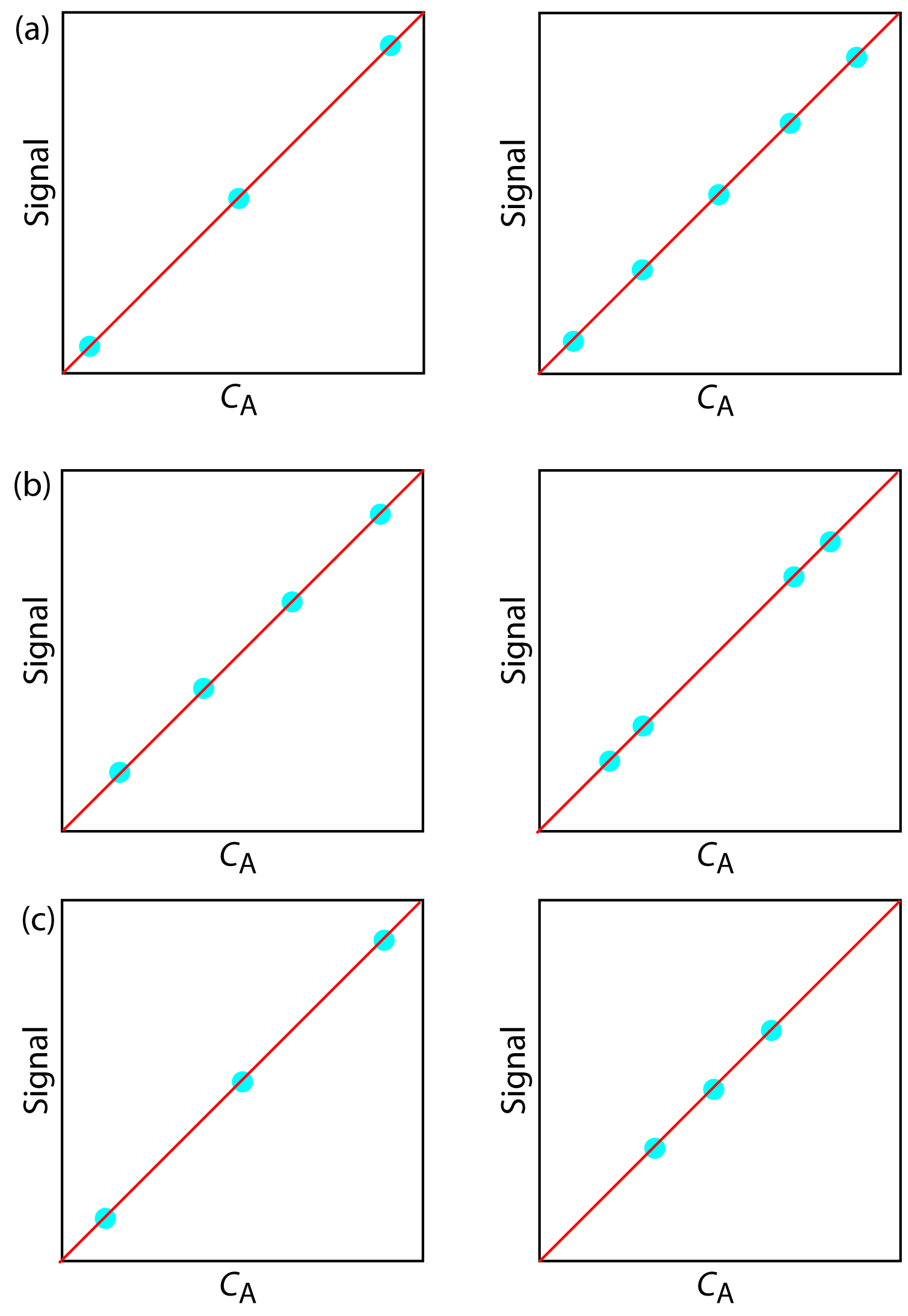
Figure 5.26 Calibration curves to accompany Problem 7.

8. The following data are for a series of external standards of Cd²⁺ buffered to a pH of 4.6.¹⁴

[Cd^2^+] (nM)	15.4	30.4	44.9	59.0	72.7	86.0
Stotal(nA)	4.8	11.4	18.2	25.6	32.3	37.7

(a) Use a linear regression to determine the standardization relationship and report confidence intervals for the slope and the y-intercept.

(b) Construct a plot of the residuals and comment on their significance.

At a pH of 3.7 the following data were recorded for the same set of external standards.

[Cd^2^+] (nM)	15.4	30.4	44.9	59.0	72.7	86.0
Stotal (nA)	15.0	42.7	58.5	77.0	101	118

(c) How much more or less sensitive is this method at the lower pH?

(d) A single sample is buffered to a pH of 3.7 and analyzed for cadmium, yielding a signal of 66.3. Report the concentration of Cd²⁺ in the sample and its 95% confidence interval.

9. To determine the concentration of analyte in a sample, a standard additions was performed. A 5.00-mL portion of sample was analyzed and then successive 0.10-mL spikes of a 600.0-mg/L standard of the analyte were added, analyzing after each spike. The following table shows the results of this analysis.

Vspike (mL)	0.00	0.10	0.20	0.30
Stotal (arbitrary units)	0.119	0.231	0.339	0.442

Construct an appropriate standard additions calibration curve and use a linear regression analysis to determine the concentration of analyte in the original sample and its 95% confidence interval.

10. Troost and Olavsesn investigated the application of an internal standardization to the quantitative analysis of polynuclear aromatic hydrocarbons.¹⁵ The following results were obtained for the analysis of phenanthrene using isotopically labeled phenanthrene as an internal standard. Each solution was analyzed twice.

CA/CIS	0.50	1.25	2.00	3.00	4.00
SA/SIS	0.514 0.522	0.993 1.024	1.486 1.471	2.044 20.80	2.342 2.550

(a) Determine the standardization relationship using a linear regression, and report confidence intervals for the slope and the y-intercept. Average the replicate signals for each standard before completing the linear regression analysis.

(b) Based on your results explain why the authors concluded that the internal standardization was inappropriate.

11. In Chapter 4 we used a paired t-test to compare two analytical methods used to independently analyze a series of samples of variable composition. An alternative approach is to plot the results for one method versus the results for the other method. If the two methods yield identical results, then the plot should have an expected slope, β₁, of 1.00 and an expected y-intercept, β₀, of 0.0. We can use a t-test to compare the slope and the y-intercept from a linear regression to the expected values. The appropriate test statistic for the y-intercept is found by rearranging equation 5.23.

\[t_\ce{exp} = \dfrac{|β_0 − b_0|}{s_{b_0}} = \dfrac{|b_0|}{s_{b_0}}\]

Rearranging equation 5.22 gives the test statistic for the slope.

\[t_\ce{exp} = \dfrac{|β_1 − b_1|}{s_{b_1}} = \dfrac{|1.00 − b_1|}{s_{b_1}}\]

Reevaluate the data in problem 25 from Chapter 4 using the same significance level as in the original problem.

Note

Although this is a common approach for comparing two analytical methods, it does violate one of the requirements for an unweighted linear regression—that indeterminate errors affect y only. Because indeterminate errors affect both analytical methods, the result of unweighted linear regression is biased. More specifically, the regression underestimates the slope, b₁, and overestimates the y-intercept, b₀. We can minimize the effect of this bias by placing the more precise analytical method on the x-axis, by using more samples to increase the degrees of freedom, and by using samples that uniformly cover the range of concentrations.

For more information, see Miller, J. C.; Miller, J. N. Statistics for Analytical Chemistry, 3rd ed. Ellis Horwood PTR Prentice-Hall: New York, 1993. Alternative approaches are found in Hartman, C.; Smeyers-Verbeke, J.; Penninckx, W.; Massart, D. L. Anal. Chim. Acta 1997, 338, 19–40, and Zwanziger, H. W.; Sârbu, C. Anal. Chem. 1998, 70, 1277–1280.

12. Consider the following three data sets, each containing values of y for the same values of x.

x 10.00 8.00 13.00 9.00 11.00 14.00 6.00 4.00 12.00 7.00 5.00

Data Set 1 y1 8.04 6.95 7.58 8.81 8.33 9.96 7.24 4.26 10.84 4.82 5.68

Data Set 2 y2 9.14 8.14 8.74 8.77 9.26 8.10 6.13 3.10 9.13 7.26 4.74

Data Set 3 y3 7.46 6.77 12.74 7.11 7.81 8.84 6.08 5.39 8.15 6.42 5.73

(a) An unweighted linear regression analysis for the three data sets gives nearly identical results. To three significant figures, each data set has a slope of 0.500 and a y-intercept of 3.00. The standard deviations in the slope and the y-intercept are 0.118 and 1.125 for each data set. All three standard deviations about the regression are 1.24, and all three data regression lines have a correlation coefficients of 0.816. Based on these results for a linear regression analysis, comment on the similarity of the data sets.

(b) Complete a linear regression analysis for each data set and verify that the results from part (a) are correct. Construct a residual plot for each data set. Do these plots change your conclusion from part (a)? Explain.

(c) Plot each data set along with the regression line and comment on your results.

(d) Data set 3 appears to contain an outlier. Remove this apparent outlier and reanalyze the data using a linear regression. Comment on your result.

(e) Briefly comment on the importance of visually examining your data.

13. Fanke and co-workers evaluated a standard additions method for a voltammetric determination of Tl.¹⁶ A summary of their results is tabulated in the following table.

ppm Tl added	Instrument Response (μA)
0.000	2.53	2.50		2.70	2.63	2.70	2.80		2.52
0.387	8.42	7.96		8.54	8.18	7.70	8.34		7.98
1.851	29.65	28.70		29.05	28.30	29.20	29.95		28.95
5.734	84.8	85.6		86.0	85.2	84.2	86.4		87.8

Use a weighted linear regression to determine the standardization relationship for this data.

5.7.3 Solutions to Practice Exercises

Practice Exercise 5.1

Substituting the sample’s absorbance into the calibration equation and solving for C_A give

\[S_\ce{samp} = 0.114 =29.59\: \ce{M}^{–1} × C_\ce{A} + 0.015\]

\[C_\ce{A} = \mathrm{3.35 × 10^{-3}\: M}\]

For the one-point standardization, we first solve for k_A

\[k_\ce{A}= \dfrac{S_\ce{std}}{C_\ce{std}} = \mathrm{\dfrac{0.0931}{3.16×10^{−3}\: M} = 29.46\: M^{−1}}\]

and then use this value of k_A to solve for C_A.

\[C_\ce{A}=\dfrac{S_\ce{samp}}{k_\ce{A}} = \mathrm{\dfrac{0.114}{29.46\: M^{−1}} = 3.87×10^{−3}\: M}\]

When using multiple standards, the indeterminate errors affecting the signal for one standard are partially compensated for by the indeterminate errors affecting the other standards. The standard selected for the one-point standardization has a signal that is smaller than that predicted by the regression equation, which underestimates k_A and overestimates C_A.

Click here to return to the chapter.

Practice Exercise 5.2

We begin with equation 5.8

\[S_\ce{spike} = k_\ce{A}\left(C_\ce{A}\dfrac{V_\ce{o}}{V_\ce{f}} + C_\ce{std}\dfrac{V_\ce{std}}{V_\ce{f}}\right)\]

rewriting it as

\[0 = \dfrac{k_\ce{A}C_\ce{A}V_\ce{o}}{V_\ce{f}} + k_\ce{A} × \left\{C_\ce{std} \dfrac{V_\ce{std}}{V_\ce{f}}\right\}\]

which is in the form of the linear equation

\[Y = y\textrm{-intercept} + \ce{slope} × X\]

where Y is S_spike and X is C_std×V_std/V_f. The slope of the line, therefore, is k_A, and the y-intercept is k_AC_AV_o/V_f. The x-intercept is the value of X when Y is zero, or

\[0 = \dfrac{k_\ce{A}C_\ce{A}V_\ce{o}}{V_\ce{f}} + k_\ce{A} × \left\{x\textrm{-intercept}\right\}\]

\[x\textrm{-intercept} = −\dfrac{\dfrac{k_\ce{A}C_\ce{A}V_\ce{o}}{V_\ce{f}}}{k_\ce{A}} = −\dfrac{C_\ce{A}V_\ce{o}}{V_\ce{f}}\]

Click here to return to the chapter.

Practice Exercise 5.3

Using the calibration equation from Figure 5.7a, we find that the x-intercept is

\[x\textrm{-intercept} = -\mathrm{\dfrac{0.1478}{0.0854\: mL^{-1}} = -1.731\: mL}\]

Plugging this into the equation for the x-intercept and solving for C_A gives the concentration of Mn²⁺ as

\[x\textrm{-intercept} = \mathrm{−3.478\: mL = - \dfrac{\mathit{C}_A × 25.00\: mL}{100.6\: mg/L} = 6.96\: mg/L}\]

For Figure 7b, the x-intercept is

\[x\textrm{-intercept} = \mathrm{−\dfrac{0.1478}{0.0425\: mL^{-1}} = −3.478\: mL}\]

and the concentration of Mn²⁺ is

\[x\textrm{-intercept} = \mathrm{−3.478\: mL = − \dfrac{\mathit{C}_A × 25.00\: mL}{50.00\: L} = 6.96\: mg/L}\]

Click here to return to the chapter.

Practice Exercise 5.4

We begin by setting up a table to help us organize the calculation.

xi	yi	xiyi	xi^2
0.000	0.00	0.000	0.000
1.55×10^–3	0.050	7.750×10^–5	2.403×10^–6
3.16×10^–3	0.093	2.939×10^–4	9.986×10^–6
4.74×10^–3	0.143	6.778×10^–4	2.247×10^–5
6.34×10^–3	0.188	1.192×10^–3	4.020×10^–5
7.92×10^–3	0.236	1.869×10^–3	6.273×10^–5

Adding the values in each column gives

\[\sum_{i}x_i = 2.371×10^{-2} \hspace{20px} \sum_{i}y_i = 0.710\]

\[\sum_{i}x_iy_i= 4.110×10^{–3} \hspace{20px} \sum_{i}x_i^2 = 1.278×10^{–4}\]

Substituting these values into equation 5.17 and equation 5.18, we find that the slope and the y-intercept are

\[b_1 = \dfrac{6×(4.110×10^{−3}) − (2.371×10^{−2})×(0.710)}{(6×1.378×10^{−4}) − (2.371×10^{−2})^2} = 29.57\]

\[b_0 = \dfrac{0.710 − 29.57×(2.371×10^{−2})}{6} = 0.0015\]

The regression equation is

\[S_\ce{std} = 29.57 × C_\ce{std} + 0.0015\]

To calculate the 95% confidence intervals, we first need to determine the standard deviation about the regression. The following table will help us organize the calculation.

xi	yi	ŷi	(yi − ŷi)^2
0.000	0.00	0.0015	2.250×10^–6
1.55×10^–3	0.050	0.0473	7.110×10^–6
3.16×10^–3	0.093	0.0949	3.768×10^–6
4.74×10^–3	0.143	0.1417	1.791×10^–6
6.34×10^–3	0.188	0.1890	9.483×10^–7
7.92×10^–3	0.236	0.2357	9.339×10^–8

Adding together the data in the last column gives the numerator of equation 5.19 as 1.596×10^–5. The standard deviation about the regression, therefore, is

\[s_r= \sqrt{\dfrac{1.596×10^{−6}}{6− 2}} = 1.997×10^{−3}\]

Next, we need to calculate the standard deviations for the slope and the y-intercept using equation 5.20 and equation 5.21.

\[s_{b_1}= \sqrt{\dfrac{6×(1.997×10^{−3})^2}{6×(1.378×10^{−4}) − (2.371×10^{−2})^2}} = 0.3007\]

\[s_{b_0}= \sqrt{\dfrac{(1.997×10^{−3})^2×(1.378×10^{−4})}{6×(1.378×10^{−4}) − (2.371×10^{−2})^2}} = 1.441×10^{−3}\]

The 95% confidence intervals are

\[β_1 = b_1 ± ts_{b_1} = \mathrm{29.57 ± (2.78×0.3007) = 29.57\: M^{-1} ± 0.85\: M^{-1}}\]

\[β_0 = b_0 ± ts_{b_0}= 0.0015 ± \left\{2.78 × (1.441×10^{−3})\right\} = 0.0015 ± 0.0040\]

With an average S_samp of 0.114, the concentration of analyte, C_A, is

\[C_\ce{A} = \dfrac{S_\ce{samp} − b_0}{b_1} = \mathrm{\dfrac{0.114− 0.0015}{29.57\: M^{-1}} = 3.80×10^{−3}\: M}\]

The standard deviation in C_A is

\[s_{C_\ce{A}}= \dfrac{1.997×10^{−3}}{29.57} \sqrt{\dfrac{1}{3} + \dfrac{1}{6} + \dfrac{(0.114−0.1183)^2}{(29.57)^2 × (4.408×10^{-5})}} = 4.778×10^{−5}\]

and the 95% confidence interval is

\[\begin{align}
\mu_{C_\ce{A}} &= C_\ce{A} ± ts_{C_\ce{A}} = 3.80×10^{−3} ± \left\{2.78×(4.778×10^{−5})\right\}\\
&= \mathrm{3.80×10^{−3}\: M ± 0.13×10^{−3}\: M}
\end{align}\]

Click here to return to the chapter.

Practice Exercise 5.5

To create a residual plot, we need to calculate the residual error for each standard. The following table contains the relevant information.

xi	yi	ŷi	yi − ŷi
0.000	0.00	0.0015	-0.0015
1.55×10^–3	0.050	0.0473	0.0027
3.16×10^–3	0.093	0.0949	-0.0019
4.74×10^–3	0.143	0.1417	0.0013
6.34×10^–3	0.188	0.1890	-0.0010
7.92×10^–3	0.236	0.2357	0.0003

Figure 5.27 shows a plot of the resulting residual errors is shown here. The residual errors appear random and do not show any significant dependence on the analyte’s concentration. Taken together, these observations suggest that our regression model is appropriate.

Figure 5.27 Plot of the residual errors for the data in Practice Exercise 5.5.

Click here to return to the chapter.

Practice Exercise 5.6

Begin by entering the data into an Excel spreadsheet, following the format shown in Figure 5.15. Because Excel’s Data Analysis tools provide most of the information we need, we will use it here. The resulting output, which is shown in Figure 5.28, contains the slope and the y-intercept, along with their respective 95% confidence intervals. Excel does not provide a function for calculating the uncertainty in the analyte’s concentration, C_A, given the signal for a sample, S_samp. You must complete these calculations by hand. With an S_samp. of 0.114, C_A

\[C_\ce{A} = \dfrac{S_\ce{samp} − b_0}{b_1} = \mathrm{\dfrac{0.114− 0.0014}{29.59\: M^{-1}} = 3.80×10^{−3}\: M}\]

The standard deviation in C_A is

\[s_{C_\ce{A}}= \dfrac{1.996×10^{−3}}{29.59} \sqrt{\dfrac{1}{3} + \dfrac{1}{6} + \dfrac{(0.114−0.1183)^2}{(29.59)^2 × (4.408×10^{-5})}} = 4.772×10^{−5}\]

and the 95% confidence interval is

\[\begin{align}
\mu_{C_\ce{A}} &= C_\ce{A} ± ts_{C_\ce{A}} = 3.80×10^{−3} ± \left\{2.78 × (4.772×10^{−5})\right\}\\
&= \mathrm{3.80×10^{−3}\: M ± 0.13×10^{−3}\: M}
\end{align}\]

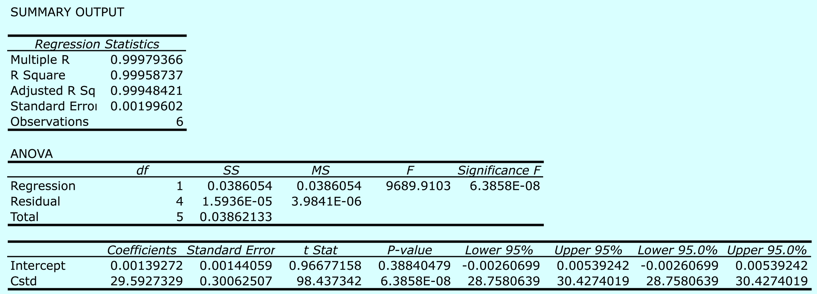
Figure 5.28 Excel’s summary of the regression results for Practice Exercise 5.6.

Click here to return to the chapter.

Practice Exercise 5.7

Figure 5.29 shows an R session for this problem, including loading the chemCal package, creating objects to hold the values for C_std, S_std, and Ssamp. Note that for Ssamp, we do not have the actual values for the three replicate measurements. In place of the actual measurements, we just enter the average signal three times. This is okay because the calculation depends on the average signal and the number of replicates, and not on the individual measurements.

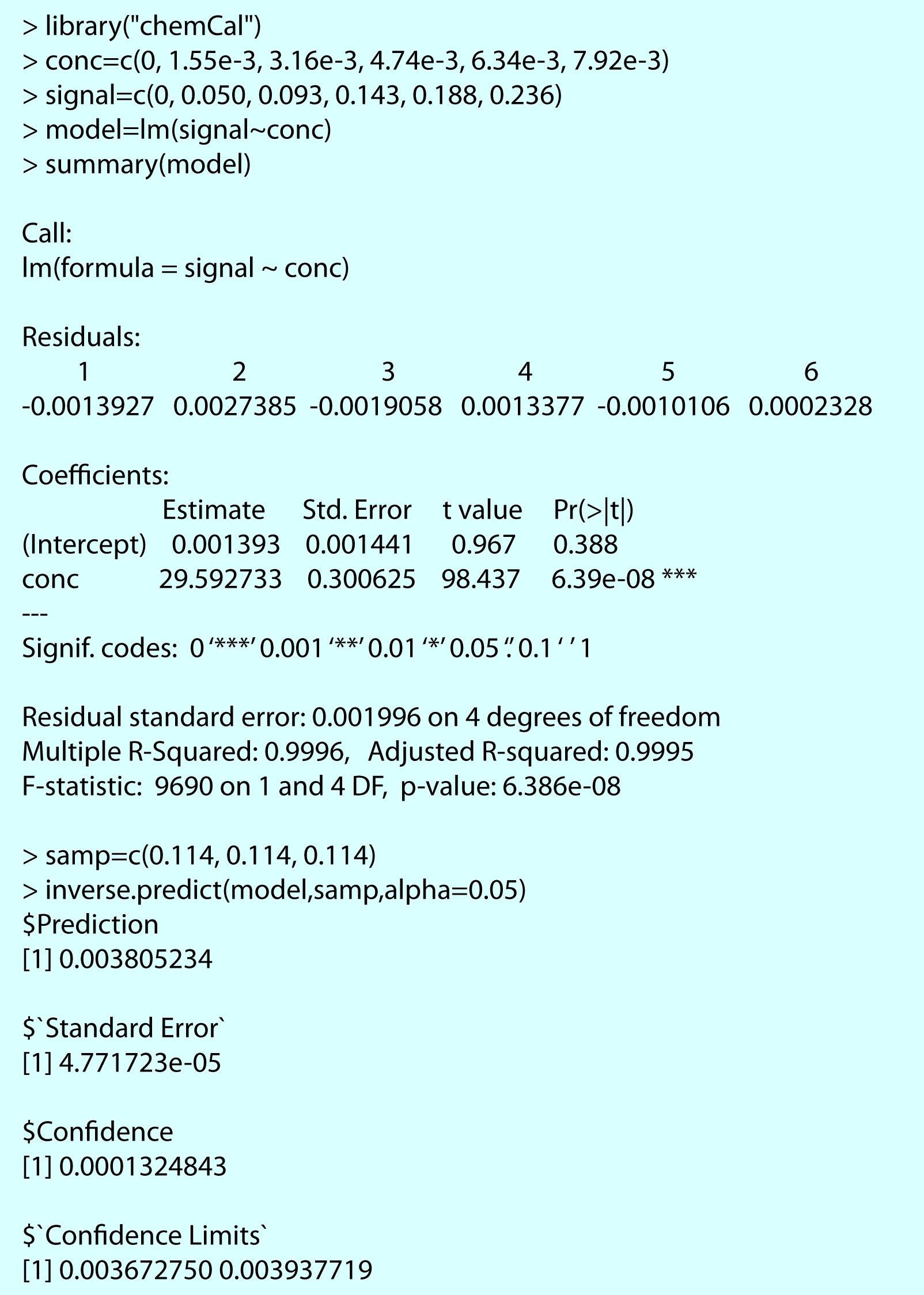
Figure 5.29 R session for completing Practice Exercise 5.7.

Click here to return to the chapter.

References

1. ACS Committee on Environmental Improvement “Guidelines for Data Acquisition and Data Quality Evaluation in Environmental Chemistry,” Anal. Chem. 1980, 52, 2242–2249.
2. (a) Smith, B. W.; Parsons, M. L. J. Chem. Educ. 1973, 50, 679–681; (b) Moody, J. R.; Greenburg, P. R.; Pratt, K. W.; Rains, T. C. Anal. Chem. 1988, 60, 1203A–1218A.
3. Committee on Analytical Reagents, Reagent Chemicals, 8th ed., American Chemical Society: Washington, D. C., 1993.
4. Ebel, S. Fresenius J. Anal. Chem. 1992, 342, 769.
5. Cardone, M. J.; Palmero, P. J.; Sybrandt, L. B. Anal. Chem. 1980, 52, 1187–1191.
6. See, for example, Draper, N. R.; Smith, H. Applied Regression Analysis, 3rd ed.; Wiley: New York, 1998.
7. (a) Miller, J. N. Analyst 1991, 116, 3–14; (b) Sharaf, M. A.; Illman, D. L.; Kowalski, B. R. Chemometrics, Wiley-Interscience: New York, 1986, pp. 126-127; (c) Analytical Methods Committee “Uncertainties in concentrations estimated from calibration experiments,” AMC Technical Brief, March 2006 (http://www.rsc.org/images/Brief22_tcm18-51117.pdf)
8. Bonate, P. J. Anal. Chem. 1993, 65, 1367–1372.
9. See, for example, Analytical Methods Committee, “Fitting a linear functional relationship to data with error on both variable,” AMC Technical Brief, March, 2002 (http://www.rsc.org/images/brief10_tcm18-25920.pdf).
10. For details about curvilinear regression, see (a) Sharaf, M. A.; Illman, D. L.; Kowalski, B. R. Chemometrics, Wiley-Interscience: New York, 1986; (b) Deming, S. N.; Morgan, S. L. Experimental Design: A Chemometric Approach, Elsevier: Amsterdam, 1987.
11. Beebe, K. R.; Kowalski, B. R. Anal. Chem. 1987, 59, 1007A–1017A.
12. Cardone, M. J. Anal. Chem. 1986, 58, 433–438.
13. Cardone, M. J. Anal. Chem. 1986, 58, 438–445.
14. Wojciechowski, M.; Balcerzak, J. Anal. Chim. Acta 1991, 249, 433–445.
15. Troost, J. R.; Olavesen, E. Y. Anal. Chem. 1996, 68, 708–711.
16. Franke, J. P.; de Zeeuw, R. A.; Hakkert, R. Anal. Chem. 1978, 50, 1374–1380.

Contributors

David Harvey (DePauw University)