12.2: General Theory of Column Chromatography

Of the two methods for bringing the stationary phase and the mobile phases into contact, the most important is column chromatography. In this section we develop a general theory that we may apply to any form of column chromatography.

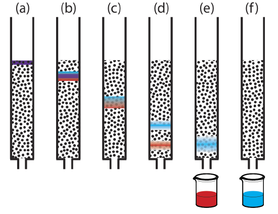
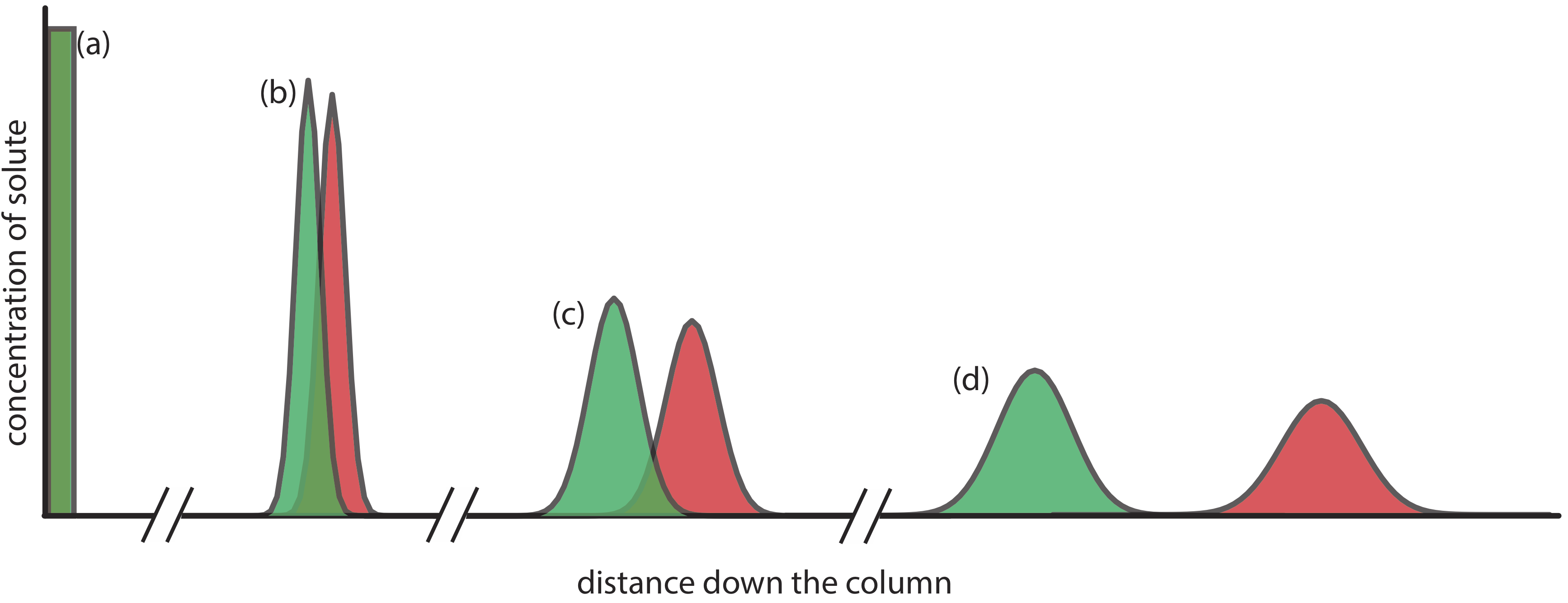
Figure \(\PageIndex{1}\) provides a simple view of a liquid–solid column chromatography experiment. The sample is introduced as a narrow band at the top of the column. Ideally, the solute’s initial concentration profile is rectangular (Figure \(\PageIndex{2}\)a). As the sample moves down the column, the solutes begin to separate (Figure \(\PageIndex{1}\)b,c) and the individual solute bands begin to broaden and develop a Gaussian profile (Figure \(\PageIndex{2}\)b,c). If the strength of each solute’s interaction with the stationary phase is sufficiently different, then the solutes separate into individual bands (Figure \(\PageIndex{1}\)d and Figure \(\PageIndex{2}\)d).

Figure \(\PageIndex{1}\). Progress of a column chromatographic separation of a two-component mixture. In (a) the sample is layered on top of the stationary phase. As mobile phase passes through the column, the sample separates into two solute bands (b–d). In (e) and (f), we collect each solute as it elutes from the column.

Figure \(\PageIndex{2}\). An alternative view of the separation in Figure \(\PageIndex{1}\) showing the concentration of each solute as a function of distance down the column.

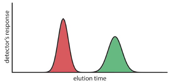
We can follow the progress of the separation by collecting fractions as they elute from the column (Figure \(\PageIndex{1}\)e,f), or by placing a suitable detector at the end of the column. A plot of the detector’s response as a function of elution time, or as a function of the volume of mobile phase, is known as a chromatogram (Figure \(\PageIndex{3}\)), and consists of a peak for each solute.

Figure \(\PageIndex{3}\). Chromatogram for the separation shown in Figure \(\PageIndex{1}\) and Figure \(\PageIndex{2}\), showing the detector’s response as a function of the elution time.

There are many possible detectors that we can use to monitor the separation. Later sections of this chapter describe some of the most popular.

We can characterize a chromatographic peak’s properties in several ways, two of which are shown in Figure \(\PageIndex{4}\). Retention time, t_r, is the time between the sample’s injection and the maximum response for the solute’s peak. A chromatographic peak’s baseline width, w, as shown in Figure \(\PageIndex{4}\), is determined by extending tangent lines from the inflection points on either side of the peak through the baseline. Although usually we report t_r and w using units of time, we can report them using units of volume by multiplying each by the mobile phase’s velocity, or report them in linear units by measuring distances with a ruler.

For example, a solute’s retention volume,V_r, is \(t_\text{r} \times u\) where u is the mobile phase’s velocity through the column.

Figure \(\PageIndex{4}\). Chromatogram showing a solute’s retention time, t_r, and baseline width, w, and the column’s void time, t_m, for nonretained solutes.

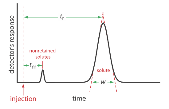
In addition to the solute’s peak, Figure \(\PageIndex{4}\) also shows a small peak that elutes shortly after the sample is injected into the mobile phase. This peak contains all nonretained solutes, which move through the column at the same rate as the mobile phase. The time required to elute the nonretained solutes is called the column’s void time, t_m.

Chromatographic Resolution

The goal of chromatography is to separate a mixture into a series of chromatographic peaks, each of which constitutes a single component of the mixture. The resolution between two chromatographic peaks, R_AB, is a quantitative measure of their separation, and is defined as

\[R_{A B}=\frac{t_{t, B}-t_{t,A}}{0.5\left(w_{B}+w_{A}\right)}=\frac{2 \Delta t_{r}}{w_{B}+w_{A}} \label{12.1}\]

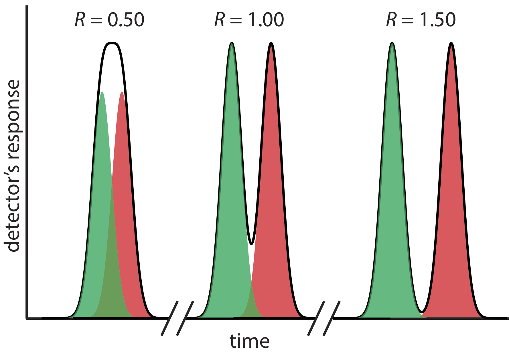
where B is the later eluting of the two solutes. As shown in Figure \(\PageIndex{5}\), the separation of two chromatographic peaks improves with an increase in R_AB. If the areas under the two peaks are identical—as is the case in Figure \(\PageIndex{5}\)—then a resolution of 1.50 corresponds to an overlap of only 0.13% for the two elution profiles. Because resolution is a quantitative measure of a separation’s success, it is a useful way to determine if a change in experimental conditions leads to a better separation.

Figure \(\PageIndex{5}\). Three examples that show the relationship between resolution and the separation of a two component mixture. The green peak and the red peak are the elution profiles for the two components. The chromatographic peak— which is the sum of the two elution profiles—is shown by the solid black line.

Example \(\PageIndex{1}\)

In a chromatographic analysis of lemon oil a peak for limonene has a retention time of 8.36 min with a baseline width of 0.96 min. \(\gamma\)-Terpinene elutes at 9.54 min with a baseline width of 0.64 min. What is the resolution between the two peaks?

Solution

Using equation \ref{12.1} we find that the resolution is

\[R_{A B}=\frac{2 \Delta t_{r}}{w_{B}+w_{A}}=\frac{2(9.54 \text{ min}-8.36 \text{ min})}{0.64 \text{ min}+0.96 \text{ min}}=1.48 \nonumber\]

Figure \(\PageIndex{6}\). Chromatogram for Exercise \(\PageIndex{1}\).

Exercise \(\PageIndex{1}\)

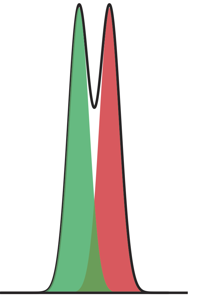
Figure \(\PageIndex{6}\) shows the separation of a two-component mixture. What is the resolution between the two components? Use a ruler to measure \(\Delta t_\text{r}\), w_A, and w_B in millimeters.

Answer

Because the relationship between elution time and distance is proportional, we can measure \(\Delta t_\text{r}\), w_A, and w_B using a ruler. My measurements are 8.5 mm for \(\Delta t_\text{r}\), and 12.0 mm each for w_A and w_B. Using these values, the resolution is

\[R_{A B}=\frac{2 \Delta t_{t}}{w_{A}+w_{B}}=\frac{2(8.5 \text{ mm})}{12.0 \text{ mm}+12.0 \text{ mm}}=0.70 \nonumber\]

Your measurements for \(\Delta t_\text{r}\), w_A, and w_B will depend on the relative size of your monitor or printout; however, your value for the resolution should be similar to the answer above.

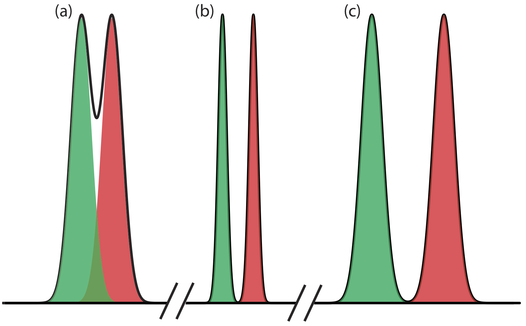
Equation \ref{12.1} suggests that we can improve resolution by increasing \(\Delta t_\text{r}\), or by decreasing w_A and w_B (Figure \(\PageIndex{7}\)). To increase \(\Delta t_\text{r}\) we can use one of two strategies. One approach is to adjust the separation conditions so that both solutes spend less time in the mobile phase—that is, we increase each solute’s retention factor—which provides more time to effect a separation. A second approach is to increase selectivity by adjusting conditions so that only one solute experiences a significant change in its retention time. The baseline width of a solute’s peak depends on the solutes movement within and between the mobile phase and the stationary phase, and is governed by several factors that collectively we call column efficiency. We will consider each of these approaches for improving resolution in more detail, but first we must define some terms.

Figure \(\PageIndex{7}\). Two method for improving chromatographic resolution: (a) original chromatogram; (b) chromatogram after decreasing w_A and w_B by \(4 \times\); and (c) chromatogram after increasing \(\Delta t_\text{r}\) by \(2 \times\).

Solute Retention Factor

Let’s assume we can describe a solute’s distribution between the mobile phase and stationary phase using the following equilibrium reaction

\[S_{\text{m}} \rightleftharpoons S_{\text{s}} \nonumber\]

where S_m is the solute in the mobile phase and S_s is the solute in the stationary phase. Following the same approach we used in Chapter 7.7 for liquid–liquid extractions, the equilibrium constant for this reaction is an equilibrium partition coefficient, K_D.

\[K_{D}=\frac{\left[S_{\mathrm{s}}\right]}{\left[S_\text{m}\right]} \nonumber\]

This is not a trivial assumption. In this section we are, in effect, treating the solute’s equilibrium between the mobile phase and the stationary phase as if it is identical to the equilibrium in a liquid–liquid extraction. You might question whether this is a reasonable assumption. There is an important difference between the two experiments that we need to consider. In a liquid–liquid extraction, which takes place in a separatory funnel, the two phases remain in contact with each other at all times, allowing for a true equilibrium. In chromatography, however, the mobile phase is in constant motion. A solute that moves into the stationary phase from the mobile phase will equilibrate back into a different portion of the mobile phase; this does not describe a true equilibrium.

So, we ask again: Can we treat a solute’s distribution between the mobile phase and the stationary phase as an equilibrium process? The answer is yes, if the mobile phase velocity is slow relative to the kinetics of the solute’s movement back and forth between the two phase. In general, this is a reasonable assumption.

In the absence of any additional equilibrium reactions in the mobile phase or the stationary phase, K_D is equivalent to the distribution ratio, D,

\[D=\frac{\left[S_{0}\right]}{\left[S_\text{m}\right]}=\frac{(\operatorname{mol} \text{S})_\text{s} / V_\text{s}}{(\operatorname{mol} \text{S})_\text{m} / V_\text{m}}=K_{D} \label{12.2}\]

where V_s and V_m are the volumes of the stationary phase and the mobile phase, respectively.

A conservation of mass requires that the total moles of solute remain constant throughout the separation; thus, we know that the following equation is true.

\[(\operatorname{mol} \text{S})_{\operatorname{tot}}=(\operatorname{mol} \text{S})_{\mathrm{m}}+(\operatorname{mol} \text{S})_\text{s} \label{12.3}\]

Solving equation \ref{12.3} for the moles of solute in the stationary phase and substituting into equation \ref{12.2} leaves us with

\[D = \frac{\left\{(\text{mol S})_{\text{tot}} - (\text{mol S})_\text{m}\right\} / V_{\mathrm{s}}}{(\text{mol S})_{\mathrm{m}} / V_{\mathrm{m}}} \nonumber\]

Rearranging this equation and solving for the fraction of solute in the mobile phase, f_m, gives

\[f_\text{m} = \frac {(\text{mol S})_\text{m}} {(\text{mol S})_\text{tot}} = \frac {V_\text{m}} {DV_\text{s} + V_\text{m}} \label{12.4}\]

which is identical to the result for a liquid-liquid extraction (see Chapter 7). Because we may not know the exact volumes of the stationary phase and the mobile phase, we simplify equation \ref{12.4} by dividing both the numerator and the denominator by V_m; thus

\[f_\text{m} = \frac {V_\text{m}/V_\text{m}} {DV_\text{s}/V_\text{m} + V_\text{m}/V_\text{m}} = \frac {1} {DV_\text{s}/V_\text{m} + 1} = \frac {1} {1+k} \label{12.5}\]

where k

\[k=D \times \frac{V_\text{s}}{V_\text{m}} \label{12.6}\]

is the solute’s retention factor. Note that the larger the retention factor, the more the distribution ratio favors the stationary phase, leading to a more strongly retained solute and a longer retention time.

Other (older) names for the retention factor are capacity factor, capacity ratio, and partition ratio, and it sometimes is given the symbol \(k^{\prime}\). Keep this in mind if you are using other resources. Retention factor is the approved name from the IUPAC Gold Book.

We can determine a solute’s retention factor from a chromatogram by measuring the column’s void time, t_m, and the solute’s retention time, t_r (see Figure \(\PageIndex{4}\)). Solving equation \ref{12.5} for k, we find that

\[k=\frac{1-f_\text{m}}{f_\text{m}} \label{12.7}\]

Earlier we defined f_m as the fraction of solute in the mobile phase. Assuming a constant mobile phase velocity, we also can define f_m as

\[f_\text{m}=\frac{\text { time spent in the mobile phase }}{\text { time spent in the stationary phase }}=\frac{t_\text{m}}{t_\text{r}} \nonumber\]

Substituting back into equation \ref{12.7} and rearranging leaves us with

\[k=\frac{1-\frac{t_{m}}{t_{t}}}{\frac{t_{\mathrm{m}}}{t_{\mathrm{r}}}}=\frac{t_{\mathrm{t}}-t_{\mathrm{m}}}{t_{\mathrm{m}}}=\frac{t_{\mathrm{r}}^{\prime}}{t_{\mathrm{m}}} \label{12.8}\]

where \(t_\text{r}^{\prime}\) is the adjusted retention time.

Example \(\PageIndex{2}\)

In a chromatographic analysis of low molecular weight acids, butyric acid elutes with a retention time of 7.63 min. The column’s void time is 0.31 min. Calculate the retention factor for butyric acid.

Solution

\[k_{\mathrm{but}}=\frac{t_{\mathrm{r}}-t_{\mathrm{m}}}{t_{\mathrm{m}}}=\frac{7.63 \text{ min}-0.31 \text{ min}}{0.31 \text{ min}}=23.6 \nonumber\]

Figure \(\PageIndex{8}\). Chromatogram for Exercise \(\PageIndex{2}\).

Exercise \(\PageIndex{2}\)

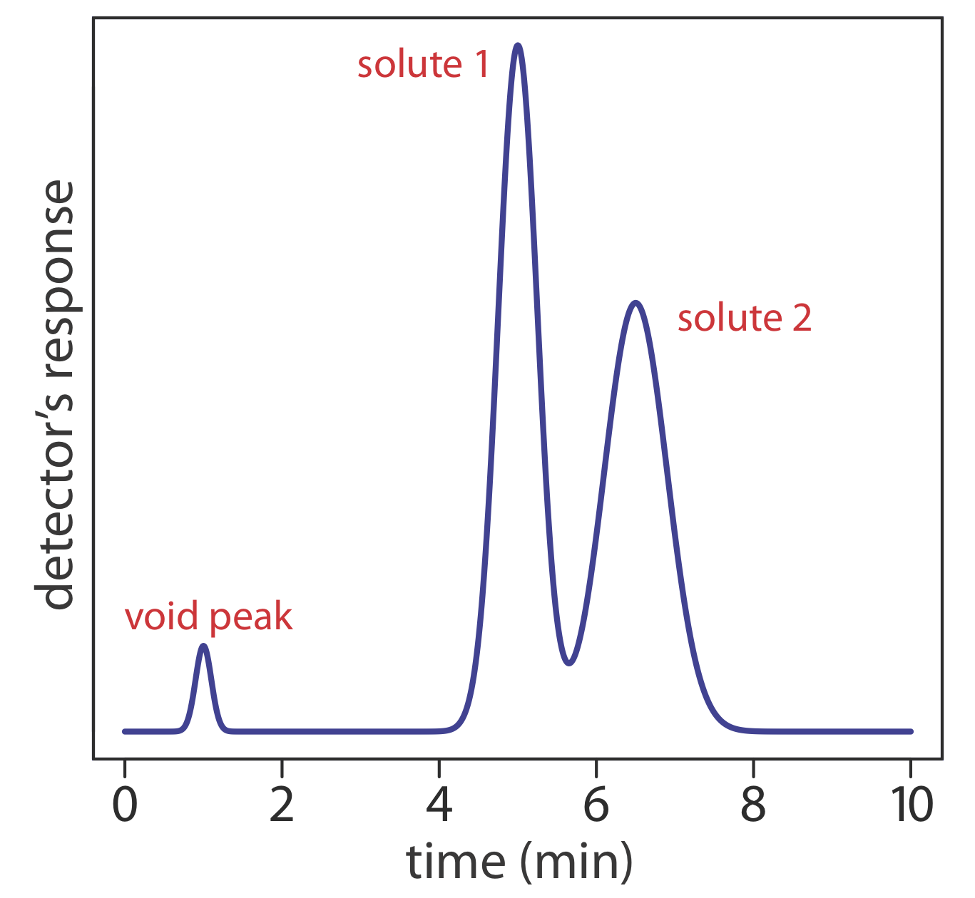
Figure \(\PageIndex{8}\) is the chromatogram for a two-component mixture. Determine the retention factor for each solute assuming the sample was injected at time t = 0.

Answer

Because the relationship between elution time and distance is proportional, we can measure t_m, t_r,1, and t_r,2 using a ruler. My measurements are 7.8 mm, 40.2 mm, and 51.5 mm, respectively. Using these values, the retention factors for solute A and solute B are

\[k_{1}=\frac{t_{\mathrm{r} 1}-t_\text{m}}{t_\text{m}}=\frac{40.2 \text{ mm}-7.8 \text{ mm}}{7.8 \text{ mm}}=4.15 \nonumber\]

\[k_{2}=\frac{t_{\mathrm{r} 2}-t_\text{m}}{t_\text{m}}=\frac{51.5 \text{ mm}-7.8 \text{ mm}}{7.8 \text{ mm}}=5.60 \nonumber\]

Your measurements for t_m, t_r,1, and t_r,2 will depend on the relative size of your monitor or printout; however, your value for the resolution should be similar to the answer above.

Selectivity

Selectivity is a relative measure of the retention of two solutes, which we define using a selectivity factor, \(\alpha\)

\[\alpha=\frac{k_{B}}{k_{A}}=\frac{t_{r, B}-t_{\mathrm{m}}}{t_{r, A}-t_{\mathrm{m}}} \label{12.9}\]

where solute A has the smaller retention time. When two solutes elute with identical retention time, \(\alpha = 1.00\); for all other conditions \(\alpha > 1.00\).

Example \(\PageIndex{3}\)

In the chromatographic analysis for low molecular weight acids described in Example \(\PageIndex{2}\), the retention time for isobutyric acid is 5.98 min. What is the selectivity factor for isobutyric acid and butyric acid?

Solution

First we must calculate the retention factor for isobutyric acid. Using the void time from Example \(\PageIndex{2}\) we have

\[k_{\mathrm{iso}}=\frac{t_{\mathrm{r}}-t_{\mathrm{m}}}{t_{\mathrm{m}}}=\frac{5.98 \text{ min}-0.31 \text{ min}}{0.31 \text{ min}}=18.3 \nonumber\]

The selectivity factor, therefore, is

\[\alpha=\frac{k_{\text {but }}}{k_{\text {iso }}}=\frac{23.6}{18.3}=1.29 \nonumber\]

Exercise \(\PageIndex{3}\)

Determine the selectivity factor for the chromatogram in Exercise \(\PageIndex{2}\).

Answer

Using the results from Exercise \(\PageIndex{2}\), the selectivity factor is

\[\alpha=\frac{k_{2}}{k_{1}}=\frac{5.60}{4.15}=1.35 \nonumber\]

Your answer may differ slightly due to differences in your values for the two retention factors.

Column Efficiency

Suppose we inject a sample that has a single component. At the moment we inject the sample it is a narrow band of finite width. As the sample passes through the column, the width of this band continually increases in a process we call band broadening. Column efficiency is a quantitative measure of the extent of band broadening.

See Figure \(\PageIndex{1}\) and Figure \(\PageIndex{2}\). When we inject the sample it has a uniform, or rectangular concentration profile with respect to distance down the column. As it passes through the column, the band broadens and takes on a Gaussian concentration profile.

In their original theoretical model of chromatography, Martin and Synge divided the chromatographic column into discrete sections, which they called theoretical plates. Within each theoretical plate there is an equilibrium between the solute present in the stationary phase and the solute present in the mobile phase [Martin, A. J. P.; Synge, R. L. M. Biochem. J. 1941, 35, 1358–1366]. They described column efficiency in terms of the number of theoretical plates, N,

\[N=\frac{L}{H} \label{12.10}\]

where L is the column’s length and H is the height of a theoretical plate. For any given column, the column efficiency improves—and chromatographic peaks become narrower—when there are more theoretical plates.

If we assume that a chromatographic peak has a Gaussian profile, then the extent of band broadening is given by the peak’s variance or standard deviation. The height of a theoretical plate is the peak’s variance per unit length of the column

\[H=\frac{\sigma^{2}}{L} \label{12.11}\]

where the standard deviation, \(\sigma\), has units of distance. Because retention times and peak widths usually are measured in seconds or minutes, it is more convenient to express the standard deviation in units of time, \(\tau\), by dividing \(\sigma\) by the solute’s average linear velocity, \(\overline{u}\), which is equivalent to dividing the distance it travels, L, by its retention time, t_r.

\[\tau=\frac{\sigma}{\overline{u}}=\frac{\sigma t_{r}}{L} \label{12.12}\]

For a Gaussian peak shape, the width at the baseline, w, is four times its standard deviation, \(\tau\).

\[w = 4 \tau \label{12.13}\]

Combining equation \ref{12.11}, equation \ref{12.12}, and equation \ref{12.13} defines the height of a theoretical plate in terms of the easily measured chromatographic parameters t_r and w.

\[H=\frac{L w^{2}}{16 t_\text{r}^{2}} \label{12.14}\]

Combing equation \ref{12.14} and equation \ref{12.10} gives the number of theoretical plates.

\[N=16 \frac{t_{\mathrm{r}}^{2}}{w^{2}}=16\left(\frac{t_{\mathrm{r}}}{w}\right)^{2} \label{12.15}\]

Example \(\PageIndex{4}\)

A chromatographic analysis for the chlorinated pesticide Dieldrin gives a peak with a retention time of 8.68 min and a baseline width of 0.29 min. Calculate the number of theoretical plates? Given that the column is 2.0 m long, what is the height of a theoretical plate in mm?

Solution

Using equation \ref{12.15}, the number of theoretical plates is

\[N=16 \frac{t_{\mathrm{r}}^{2}}{w^{2}}=16 \times \frac{(8.68 \text{ min})^{2}}{(0.29 \text{ min})^{2}}=14300 \text{ plates} \nonumber\]

Solving equation \ref{12.10} for H gives the average height of a theoretical plate as

\[H=\frac{L}{N}=\frac{2.00 \text{ m}}{14300 \text{ plates}} \times \frac{1000 \text{ mm}}{\mathrm{m}}=0.14 \text{ mm} / \mathrm{plate} \nonumber\]

Exercise \(\PageIndex{4}\)

For each solute in the chromatogram for Exercise \(\PageIndex{2}\), calculate the number of theoretical plates and the average height of a theoretical plate. The column is 0.5 m long.

Answer

Because the relationship between elution time and distance is proportional, we can measure t_r,1, t_r,2, w₁, and w₂ using a ruler. My measurements are 40.2 mm, 51.5 mm, 8.0 mm, and 13.5 mm, respectively. Using these values, the number of theoretical plates for each solute is

\[N_{1}=16 \frac{t_{r,1}^{2}}{w_{1}^{2}}=16 \times \frac{(40.2 \text{ mm})^{2}}{(8.0 \text{ mm})^{2}}=400 \text { theoretical plates } \nonumber\]

\[N_{2}=16 \frac{t_{r,2}^{2}}{w_{2}^{2}}=16 \times \frac{(51.5 \text{ mm})^{2}}{(13.5 \text{ mm})^{2}}=233 \text { theoretical plates } \nonumber\]

The height of a theoretical plate for each solute is

\[H_{1}=\frac{L}{N_{1}}=\frac{0.500 \text{ m}}{400 \text { plates }} \times \frac{1000 \text{ mm}}{\mathrm{m}}=1.2 \text{ mm} / \mathrm{plate} \nonumber\]

\[H_{2}=\frac{L}{N_{2}}=\frac{0.500 \text{ m}}{233 \text { plates }} \times \frac{1000 \text{ mm}}{\mathrm{m}}=2.15 \text{ mm} / \mathrm{plate} \nonumber\]

Your measurements for t_r,1, t_r,2, w₁, and w₂ will depend on the relative size of your monitor or printout; however, your values for N and for H should be similar to the answer above.

It is important to remember that a theoretical plate is an artificial construct and that a chromatographic column does not contain physical plates. In fact, the number of theoretical plates depends on both the properties of the column and the solute. As a result, the number of theoretical plates for a column may vary from solute to solute.

Peak Capacity

One advantage of improving column efficiency is that we can separate more solutes with baseline resolution. One estimate of the number of solutes that we can separate is

\[n_{c}=1+\frac{\sqrt{N}}{4} \ln \frac{V_{\max }}{V_{\min }} \label{12.16}\]

where n_c is the column’s peak capacity, and V_min and V_max are the smallest and the largest volumes of mobile phase in which we can elute and detect a solute [Giddings, J. C. Unified Separation Science, Wiley-Interscience: New York, 1991]. A column with 10 000 theoretical plates, for example, can resolve no more than

\[n_{c}=1+\frac{\sqrt{10000}}{4} \ln \frac{30 \mathrm{mL}}{1 \mathrm{mL}}=86 \text { solutes } \nonumber\]

if V_min and V_max are 1 mL and 30 mL, respectively. This estimate provides an upper bound on the number of solutes and may help us exclude from consideration a column that does not have enough theoretical plates to separate a complex mixture. Just because a column’s theoretical peak capacity is larger than the number of solutes, however, does not mean that a separation is feasible. In most situations the practical peak capacity is less than the theoretical peak capacity because the retention characteristics of some solutes are so similar that a separation is impossible. Nevertheless, columns with more theoretical plates, or with a greater range of possible elution volumes, are more likely to separate a complex mixture.

The smallest volume we can use is the column’s void volume. The largest volume is determined either by our patience—the maximum analysis time we can tolerate—or by our inability to detect solutes because there is too much band broadening.

Asymmetric Peaks

Our treatment of chromatography in this section assumes that a solute elutes as a symmetrical Gaussian peak, such as that shown in Figure \(\PageIndex{4}\). This ideal behavior occurs when the solute’s partition coefficient, K_D

\[K_{\mathrm{D}}=\frac{[S_\text{s}]}{\left[S_\text{m}\right]} \nonumber\]

is the same for all concentrations of solute. If this is not the case, then the chromatographic peak has an asymmetric peak shape similar to those shown in Figure \(\PageIndex{9}\). The chromatographic peak in Figure \(\PageIndex{9}\)a is an example of peak tailing, which occurs when some sites on the stationary phase retain the solute more strongly than other sites. Figure \(\PageIndex{9}\)b, which is an example of peak fronting most often is the result of overloading the column with sample.

Figure \(\PageIndex{9}\). Examples of asymmetric chromatographic peaks showing (a) peak tailing and (b) peak fronting. For both (a) and (b) the green chromatogram is the asymmetric peak and the red dashed chromatogram shows the ideal, Gaussian peak shape. The insets show the relationship between the concentration of solute in the stationary phase, [S]_s, and its concentration in the mobile phase, [S]_m. The dashed red lines show ideal behavior (K_D is constant for all conditions) and the green lines show nonideal behavior (K_D decreases or increases for higher total concentrations of solute). A quantitative measure of peak tailing, T, is shown in (a).

As shown in Figure \(\PageIndex{9}\)a, we can report a peak’s asymmetry by drawing a horizontal line at 10% of the peak’s maximum height and measuring the distance from each side of the peak to a line drawn vertically through the peak’s maximum. The asymmetry factor, T, is defined as

\[T=\frac{b}{a} \nonumber\]

The number of theoretical plates for an asymmetric peak shape is approximately

\[N \approx \frac{41.7 \times \frac{t_{r}^{2}}{\left(w_{0.1}\right)^{2}}}{T+1.25}=\frac{41.7 \times \frac{t_{r}^{2}}{(a+b)^{2}}}{T+1.25} \nonumber\]

where w_0.1 is the width at 10% of the peak’s height [Foley, J. P.; Dorsey, J. G. Anal. Chem. 1983, 55, 730–737].

Asymmetric peaks have fewer theoretical plates, and the more asymmetric the peak the smaller the number of theoretical plates. For example, the following table gives values for N for a solute eluting with a retention time of 10.0 min and a peak width of 1.00 min.

b	a	T	N
0.5	0.5	1.00	1850
0.6	0.4	1.50	1520
0.7	0.3	2.33	1160
0.8	0.2	4.00	790